Scaricare la presentazione
La presentazione è in caricamento. Aspetta per favore

1
Next Generation Sequencing
Giulio Pavesi University of Milano

4
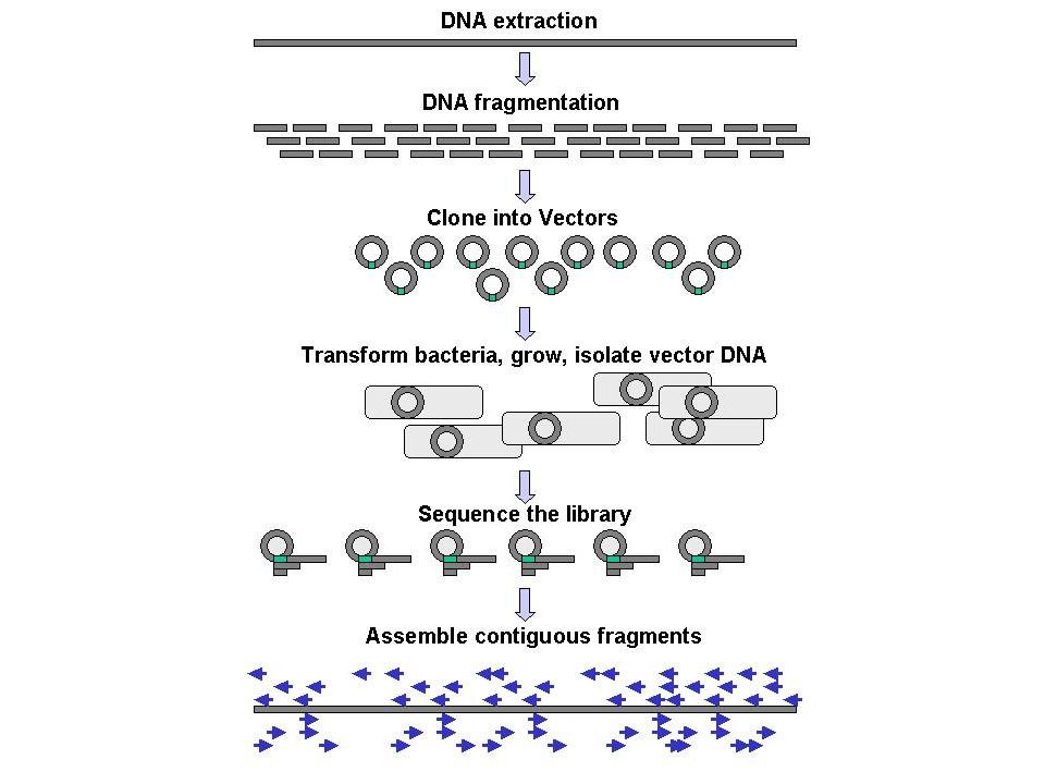
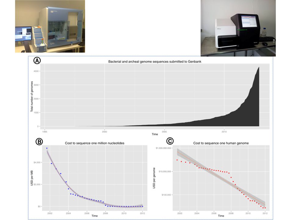
Next generation sequencing vs Sanger sequencing

6
Next Generation Sequencing
Applicazioni: Sequenziamento de novo di genomi Risequenziamento di genomi per identificazione di varianti Metagenomica Sequenziamento e quantificazione di trascrittomi Sequenziamento di “campioni” di DNA/RNA (estratti secondo diversi criteri)
")
7
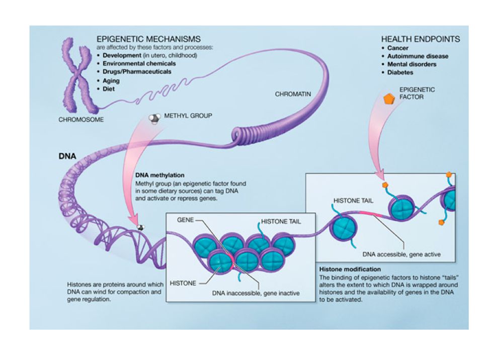
“Epigenetica” L'epigenetica (dal greco επί, epì = "sopra" e γεννετικός, gennetikòs = "relativo all'eredità familiare") si riferisce a quei cambiamenti che influenzano il fenotipo senza alterare il genotipo, ed è una branca della genetica che descrive tutte quelle modificazioni ereditabili che variano l’espressione genica pur non alterando la sequenza del DNA Che cosa c’entra il sequenziamento del DNA con qualcosa che *non* riguarda la sequenza del DNA?!?!?!
 si riferisce a quei cambiamenti che influenzano il fenotipo senza alterare il genotipo, ed è una branca della genetica che descrive tutte quelle modificazioni ereditabili che variano l’espressione genica pur non alterando la sequenza del DNA. Che cosa c’entra il sequenziamento del DNA con qualcosa che *non* riguarda la sequenza del DNA ! ! !")
10
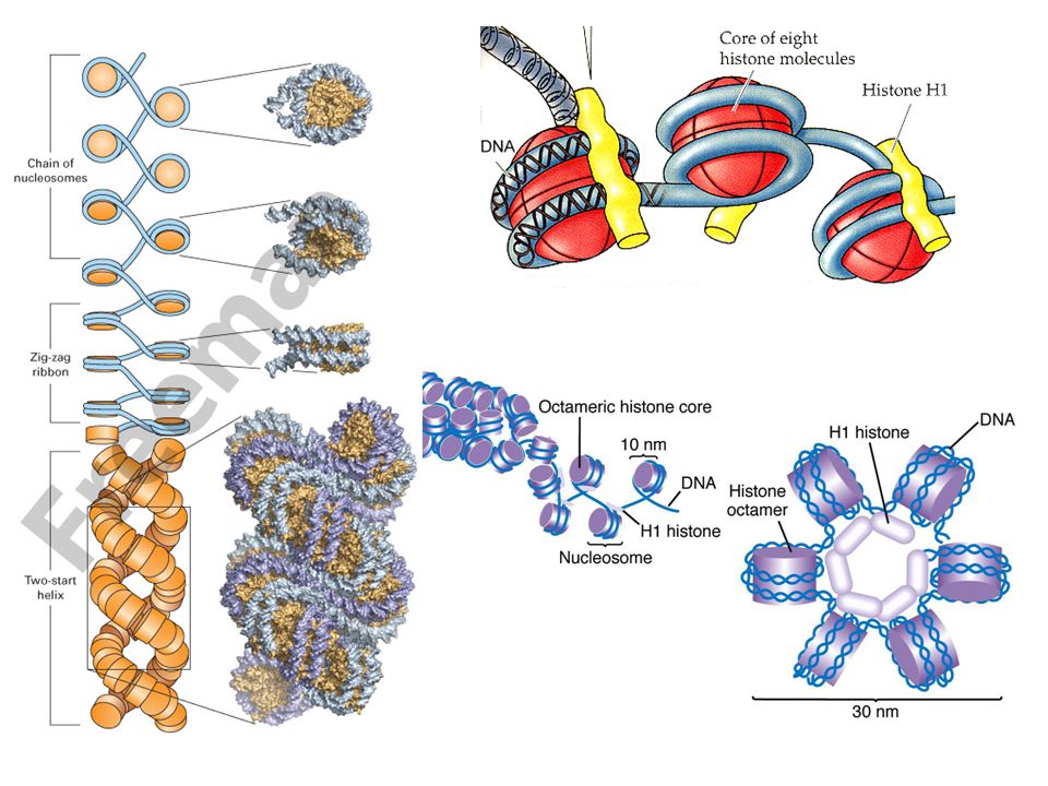
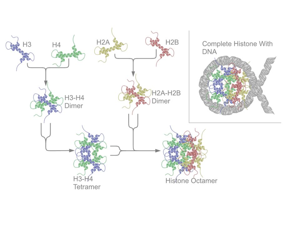
“Nucleosome” The nucleosome core particle consists of approximately 147 base pairs of DNA wrapped in 1.67 left-handed superhelical turns around a histone octamer Octamer: 2 copies each of the core histones H2A, H2B, H3, and H4 Core particles are connected by stretches of "linker DNA", which can be up to about 80 bp long

12
The histone code Example H3K4me3 H3 is the histone
K4 is the residue that is modified and its position (K lysine in position 4 of the sequence) me3 is the modification (three-methyl groups attached to K4) If no number at the end like in H3K9ac means only one group
 me3 is the modification (three-methyl groups attached to K4) If no number at the end like in H3K9ac means only one group.")
13
Different chromatin states
Chromatin structure (and thus, gene expression) depend also on the post-translational modifications associated with histones forming nuclesomes
 depend. also on the post-translational modifications associated. with histones forming nuclesomes.")
15
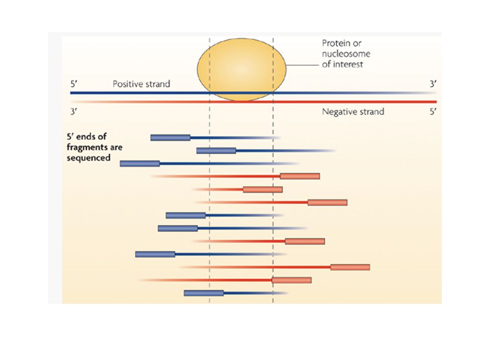
“ChIP” If we have the “right” antibody, we can extract (“immunoprecipitate”) from living cells the protein of interest bound to the DNA And - we can try to identify which were the DNA regions bound by the protein Can be done for transcription factors But can be done also for histones - and separately for each modification

16
ChIP-Seq Histone ChIP TF ChIP

17
Many cells- many copies of the same region bound by the protein

18
After ChIP Size selection: only fragments of the “right size” (200 bp)
are kept Identification of the DNA fragment bound by the protein Sequencing

19
So - if we found that a region has been sequenced many times, then we can suppose that it was bound by the protein, but…

20
Only a short fragment of the extracted DNA region can
be sequenced, at either or both ends (“single” vs “paired end” sequencing) for no more than 35 (before) / 50 (yesterday) / 100 (now) bps Thus, original regions have to be “reconstructed”
 for no more than. 35 (before) / 50 (yesterday) / 100 (now) bps. Thus, original regions have to be reconstructed")
23
Read Mapping Each sequence read has to be assigned to its original position in the genome A typical ChIP-Seq experiment produces from 6 (before) to 100 million (now) reads of and more base pairs for each sequencing “lane” (Solexa/Illumina) There exist efficient “sequence mappers” against the genome for NGS read
 to 100 million (now) reads of and more base pairs for each sequencing lane (Solexa/Illumina) There exist efficient sequence mappers against the genome for NGS read.")
24
Read Mapping “Typical” Output
@12_10_2007_SequencingRun_3_1_119_647 (actual sequence) TTTGAATATATTGAGAAAATATGACCATTTTT +12_10_2007_SequencingRun_3_1_119_647 (“quality” scores)
 TTTGAATATATTGAGAAAATATGACCATTTTT. +12_10_2007_SequencingRun_3_1_119_647 ( quality scores)")
25
“Peak finding” The critical part of any ChIP-Seq analysis is the identification of the genomic regions that produced a significantly high number of sequence reads, corresponding to the region where the protein (nucleosome) of interest was bound to DNA Since a graphical visualization of the “piling” of read mapping on the genome produces a “peak” in correspondence of these regions, the problem is often referred to as “peak finding” A “peak” then marks the region that was enriched in the original DNA sample
 of interest was bound to DNA. Since a graphical visualization of the piling of read mapping on the genome produces a peak in correspondence of these regions, the problem is often referred to as peak finding A peak then marks the region that was enriched in the original DNA sample.")
26
“Peak finding” Peaks: How tall? How wide? How much enriched?

27
“Peak finding” The main issue: the DNA sample sequenced (apart from sequencing errors/artifacts) contains a lot of “noise” Sample “contamination” - the DNA of the PhD student performing the experiment DNA shearing is not uniform: open chromatin regions tend to be fragmented more easily and thus are more likely to be sequenced Repetitive sequences might be artificially enriched due to inaccuracies in genome assembly Amplification pushed too much: you see a single DNA fragment amplified, not enriched As yet unknown problems, that anyway seem to produce “noisy” sequencings and screw the experiment up

28
ChIP-Seq histone data Histone modifications tend to be located at preferred locations with respect to gene annotations/transcribed regions Hence, enrichment can be assessed in two ways Enrichment with respect a the control experiment and peak identification “Local” enrichment in given regions with respect to gene annotations Promoters (active/non active) Upstream of transcribed/non transcribed genes Within transcribed/not transcribed regions Enhancers, whatever else
 Upstream of transcribed/non transcribed genes. Within transcribed/not transcribed regions. Enhancers, whatever else.")
29
Esperimento Eseguire una ChIP-Seq per diverse modificazioni istoniche, partendo da quelle più “classiche” Verificare: Se ciascuna modifica ha una sua localizzazione “preferenziale” sul genoma o rispetto ai geni (es. nel promotore, nella regione trascritta, etc.) Se ciascuna modifica è “correlata” in qualche modo alla trascrizione/espressione dei geni
 Se ciascuna modifica è correlata in qualche modo alla trascrizione/espressione dei geni.")
30
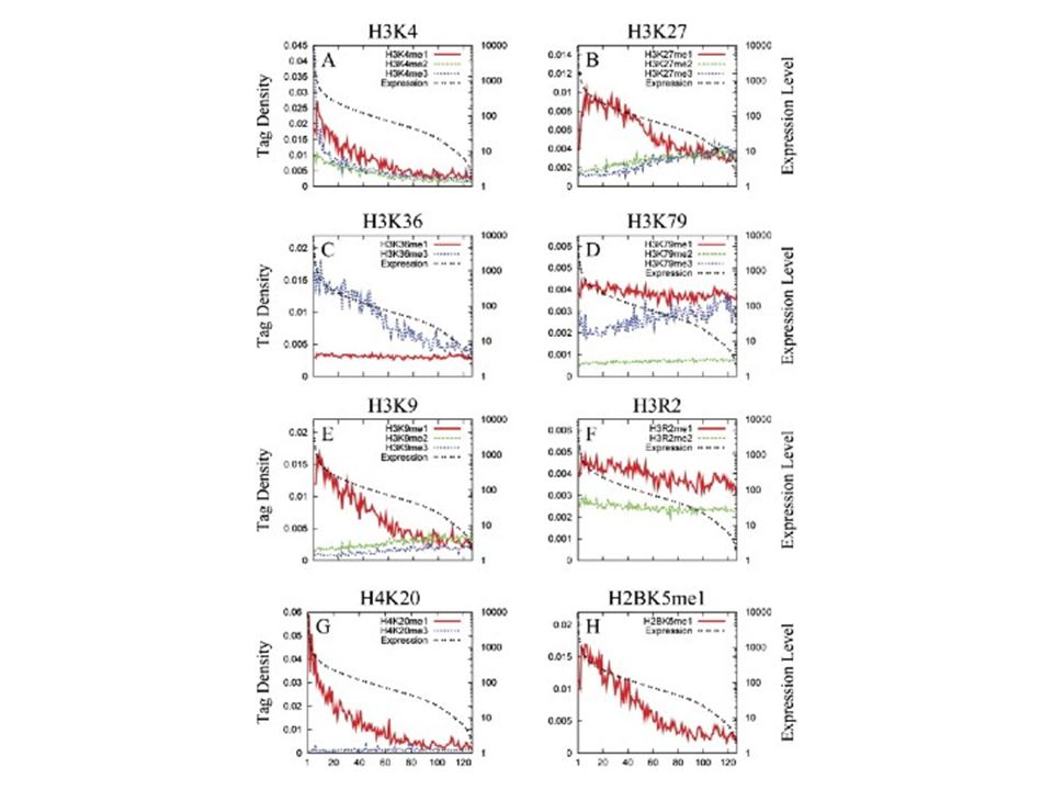
Genome wide histone modifications maps through ChIP-Seq
Barski et.al - Cell , 2007 20 histone lysine and arginine methylations in CD4+ T cells H3K27 H3K9 H3K36 H3K79 H3R2 H4K20 H4R3 H2BK5 Plus: Pol II binding H2A.Z (replaces H2A in some nucleosomes) insulator-binding protein (CTCF)
 insulator-binding protein (CTCF)")
31
Genome wide histone modifications maps through ChIP-Seq

33
Esperimento ChIP-Seq associata a una particolare modificazione (es, H3K4me3) Domanda: la modificazione è “correlabile” alla trascrizione dei geni? Ovvero, la modificazione “marca” particolari nucleosomi rispetto all’inizio della trascrizione, o alla regione trascritta Esempio: potrebbero esserci modificazioni che: Marcano l’inizio della trascrizione Marcano tutta e solo la regione trascritta “Silenziano” particolari loci genici impedendo la trascrizione Non c’entrano nulla con la trascrizione vera e propria e sono localizzate altrove

34
Esperimento Sequenze ottenute da ChIP-Seq per la modificazione studiata Input: coordinate genomiche delle posizioni in ciascuna delle sequenze mappa (vedi file di esempio) Input: coordinate genomiche dei geni RefSeq annotati Un nucleosoma marcato dalla modificazione dovrebbe corrispondere a un “mucchietto” di read che si sovrappongono (“picco”) Andiamo a contare, nucleosoma per nucleosoma, quanto alto è il “mucchietto”, ovvero quanti read sono associabili al nucleosoma
 Input: coordinate genomiche dei geni RefSeq annotati. Un nucleosoma marcato dalla modificazione dovrebbe corrispondere a un mucchietto di read che si sovrappongono ( picco ) Andiamo a contare, nucleosoma per nucleosoma, quanto alto è il mucchietto , ovvero quanti read sono associabili al nucleosoma.")
35
Esempio: se si trovasse la modifica nel nucleosoma a monte
del TSS dei geni trascritti, troveremmo un “mucchietto” così Modificazione Nucleosoma

36
Esempio: se si trovasse la modifica nei nucleosomi associati
alle regioni trascritte, troveremmo “mucchietti” così Modificazione Nucleosoma

37
“Inizi della trascrizione”
Tecniche di laboratorio come il “CAGE” (Cap-Analysis-Gene-Expression) permettono: L’esatta mappatura del 5’ degli RNA sul genoma, ovvero localizzare gli esatti TSS Quantificare il livello di trascritto prodotto a partire da ciascuno del TSS identificati Poiché cerchiamo la precisa localizzazione delle modifiche istoniche rispetto ai TSS, è importante localizzare anche i TSS con precisione
 permettono: L’esatta mappatura del 5’ degli RNA sul genoma, ovvero localizzare gli esatti TSS. Quantificare il livello di trascritto prodotto a partire da ciascuno del TSS identificati. Poiché cerchiamo la precisa localizzazione delle modifiche istoniche rispetto ai TSS, è importante localizzare anche i TSS con precisione.")
38
Analisi: primo esempio
Input Lista ordinata delle coordinate genomiche dei TSS , con relativo livello di trascritto Lista ordinata delle coordinate genomiche dove mappa ciascuna sequenza della ChIP-Seq Output: calcolare la distribuzione (i “mucchietti”) rispetto ai TSS Suddividere i TSS sulla base del livello di trascritto: Geni trascritti Geni (poco trascritti) Geni NON trascritti E verificare se ci sono differenze evidenti a seconda del fatto che il TSS sia effettivamente trascritto o meno Confrontare i risultati della modifica istonica con un esperimento di controllo
 rispetto ai TSS. Suddividere i TSS sulla base del livello di trascritto: Geni trascritti. Geni (poco trascritti) Geni NON trascritti. E verificare se ci sono differenze evidenti a seconda del fatto che il TSS sia effettivamente trascritto o meno. Confrontare i risultati della modifica istonica con un esperimento di controllo.")
39
Algoritmo! -1000 +1000 TSS Dato ciascun TSS, calcolare quante sequenze mappano tra -1000 e bp rispetto al TSS Contare quante sequenze mappano a -1000, -999, ,0 +1,+2, ,+999,+1000 Sommare per tutti i TSS i conteggi a ciascuna distanza (-1000, -999, -998,...,-1,0,+1,+2, ,+999,+1000)
")
40
Attenzione! -1000 +1000 TSS +1000 -1000 TSS
Le coordinate rispetto al TSS dipendono dalla direzione della trascrizione!!

41
Output: histone modifications at TSS
Read count (peak height) -1000 +1000 Distance from TSS
 Distance from TSS.")
42
Output: histone modifications at TSS
Read count (peak height) -1000 +1000 Distance from TSS
 Distance from TSS.")
43
PolII is found bound to DNA at the TSS of transcribed genes

44
H3K4me3 is found just before and after the TSS of transcribed genes

46
H3K4me2 (not me3!) is found just before and after the TSS of transcribed genes,
but farther away than H3K4me3

47
H3K4me1 is found just before and after the TSS of transcribed genes,
but farther away than H3K4me3 and H3K4me2

48
H3K27me3 covers the whole locus of “silent” genes - no transcription here

49
H3K27me1 (not me3!) is vice versa associated before and after loci of
transcribed genes

50
H3K36me3 is found within the transcribed region - a bit downstream of the TSS -
as if it “lets” polymerase proceed with transcription

51
H3K9me1 is similar in profile to H3K4me3

52
Barski et. al. High-Resolution Profiling of Histone Methylations in the Human Genome, Cell 129(4)
")
53
Histone modifications at transcribed regions
Read count (peak height) High Low Expression level
 High. Low. Expression level.")
55
Top: profiles for nine chromatin marks (greyscale) are shown across the WLS gene in four cell types, and summarized in a single chromatin state annotation track for each (coloured according to b). WLS is poised in ESCs, repressed in GM12878 and transcribed in HUVEC and NHLF. Its TSS switches accordingly between poised (purple), repressed (grey) and active (red) promoter states; enhancer regions within the gene body become activated (orange, yellow); and its gene body changes from low signal (white) to transcribed (green). These chromatin state changes summarize coordinated changes in many chromatin marks; for example, H3K27me3, H3K4me3 and H3K4me2 jointly mark a poised promoter, whereas loss of H3K27me3 and gain of H3K27ac and H3K9ac mark promoter activation. WCE, whole-cell extract. Bottom: nine chromatin state tracks, one per cell type, in a 900-kb region centred at WLS, summarizing 90 chromatin tracks in directly interpretable dynamic annotations and showing activation and repression patterns for six genes and hundreds of regulatory regions, including enhancer states. b, Chromatin states learned jointly across cell types by a multivariate hidden Markov model. The table shows emission parameters learned de novo on the basis of genome-wide recurrent combinations of chromatin marks. Each entry denotes the frequency with which a given mark is found at genomic positions corresponding to the chromatin state. c, Genome coverage, functional enrichments and candidate annotations for each chromatin state. Blue shading indicates intensity, scaled by column. CNV, copy number variation; GM, GM d, Box plots depicting enhancer activity for predicted regulatory elements. Sequences 250 bp long corresponding either to strong or weak/poised HepG2 enhancer elements or to GM12878-specific strong enhancer elements were inserted upstream of a luciferase gene and transfected into HepG2. Reporter activity was measured in relative light units. Robust activity is seen for strong enhancers in the matched cell type, but not for weak/poised enhancers or for strong enhancers specific to a different cell type. Boxes indicate 25th, 50th and 75th percentiles, and whiskers indicate 5th and 95th percentiles.
, repressed (grey) and active (red) promoter states; enhancer regions within the gene body become activated (orange, yellow); and its gene body changes from low signal (white) to transcribed (green). These chromatin state changes summarize coordinated changes in many chromatin marks; for example, H3K27me3, H3K4me3 and H3K4me2 jointly mark a poised promoter, whereas loss of H3K27me3 and gain of H3K27ac and H3K9ac mark promoter activation. WCE, whole-cell extract. Bottom: nine chromatin state tracks, one per cell type, in a 900-kb region centred at WLS, summarizing 90 chromatin tracks in directly interpretable dynamic annotations and showing activation and repression patterns for six genes and hundreds of regulatory regions, including enhancer states. b, Chromatin states learned jointly across cell types by a multivariate hidden Markov model. The table shows emission parameters learned de novo on the basis of genome-wide recurrent combinations of chromatin marks. Each entry denotes the frequency with which a given mark is found at genomic positions corresponding to the chromatin state. c, Genome coverage, functional enrichments and candidate annotations for each chromatin state. Blue shading indicates intensity, scaled by column. CNV, copy number variation; GM, GM d, Box plots depicting enhancer activity for predicted regulatory elements. Sequences 250 bp long corresponding either to strong or weak/poised HepG2 enhancer elements or to GM12878-specific strong enhancer elements were inserted upstream of a luciferase gene and transfected into HepG2. Reporter activity was measured in relative light units. Robust activity is seen for strong enhancers in the matched cell type, but not for weak/poised enhancers or for strong enhancers specific to a different cell type. Boxes indicate 25th, 50th and 75th percentiles, and whiskers indicate 5th and 95th percentiles..")
Presentazioni simili