Uso di Genome Browser per l'annotazione di sequenze genomiche.

Presentazione sul tema: "Uso di Genome Browser per l'annotazione di sequenze genomiche."— Transcript della presentazione:

1 Uso di Genome Browser per l'annotazione di sequenze genomiche.
Allineamento di sequenze trascritte con sequenze genomiche: BLAT.

2 Febbraio 2001: Pubblicazione prime analisi sul genoma completo
PROGETTO GENOMA UMANO Milestones: 1990: Inizio (U.S. Department of Energy and the National Institutes of Health) Giugno 2000: Completamento della sequenza “working draft” dell’intero genoma umano Febbraio 2001: Pubblicazione prime analisi sul genoma completo Aprile 2003: Completamento della sequenza

3 Una sequenza viene detta “finita” quando presenta un livello di errore inferiore a 1/10000 basi e non ha gaps. Il Progetto Genoma Umano era complesso dal punto di vista tecnico ma anche dal punto di vista computazionale. L’output di una singola reazione di sequenza (read) = bp  Tutti i singoli frammenti dovevano essere assemblati in una singola stringa lineare. NCBI fornisce ora l’assembly di riferimento per i 3 principali “portali genomici”: MapView Ensembl Genome Browser

4 Annotazione del genoma
La sequenza primaria del genoma non è sufficiente… Annotazione del genoma E’ necessario riportare sull’assembly le informazioni e i dati sperimentali già ottenuti. Riconciliare e integrare l’assembly con le mappe fisiche, genetiche e citogenetiche Gli STS sono mappati sulla sequenza usando e-PCR La corrispondenza con la mappa citogenetica utilizzando FISH sistematica di BAC. L’annotazione dei geni è attuata con metodi leggermente diversi dai 3 “genome browser” L’NCBI allinea mRNA di RefSeq, mRNA di GenBank utilizzando MegaBlast. Ensembl allinea tutte le proteine umane note di SP/Trembl utilizzando un suo algoritmo UCSC allinea mRNA di Refseq e GenBank e dalle ultime release SP/Trembl con BLAT

5 Annotazione dei geni ab initio, in base a “sensori”, funzioni che tentano di dedurre la presenza di una caratteristica genica in base a motivi o proprietà statistiche del DNA. Sensori per TSS (G+C) Sensori per siti splicing (AG-GT) Sensori che misurano la composizione in basi di esoni putativi L’output dei vari sensori è combinato per generare un “modello genico” metodi basati sulla similarità: l’allineamento di una regione genomica con un cDNA o un EST sono una buona evidenza. Lo splicing alternativo complica l’interpretazione degli allineamenti tra DNA genomico, cDNA e ESTs I dati di similarità sono incompleti: trascritti poco espressi o espressi transientemente sono assenti… I programmi di ultima generazione come Grail/Exp, Genie EST, GenomeScan combinano predizioni ab inizio con dati di similarità ottenendo risultati migliori

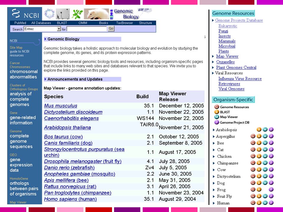
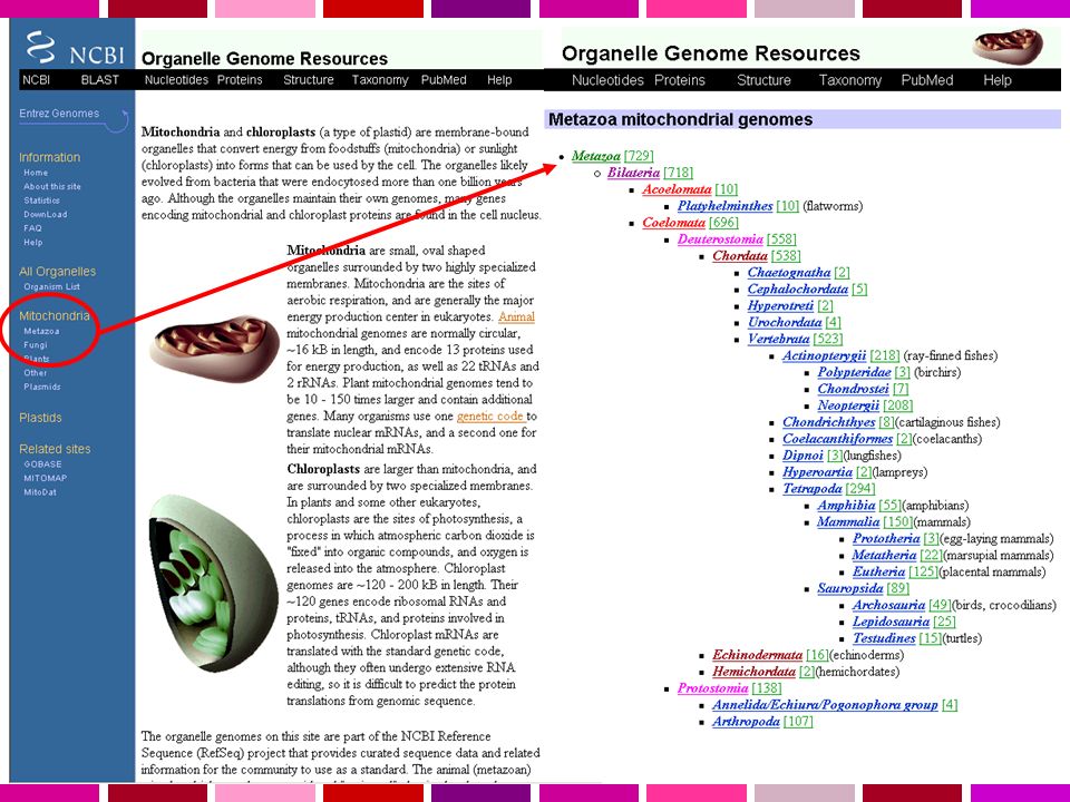
6 Viral Genomes

7

8

9

10

11

12

13 3 milioni di basi in formato testo = nessuna utilita’
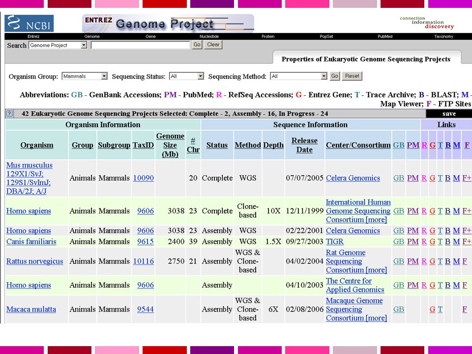
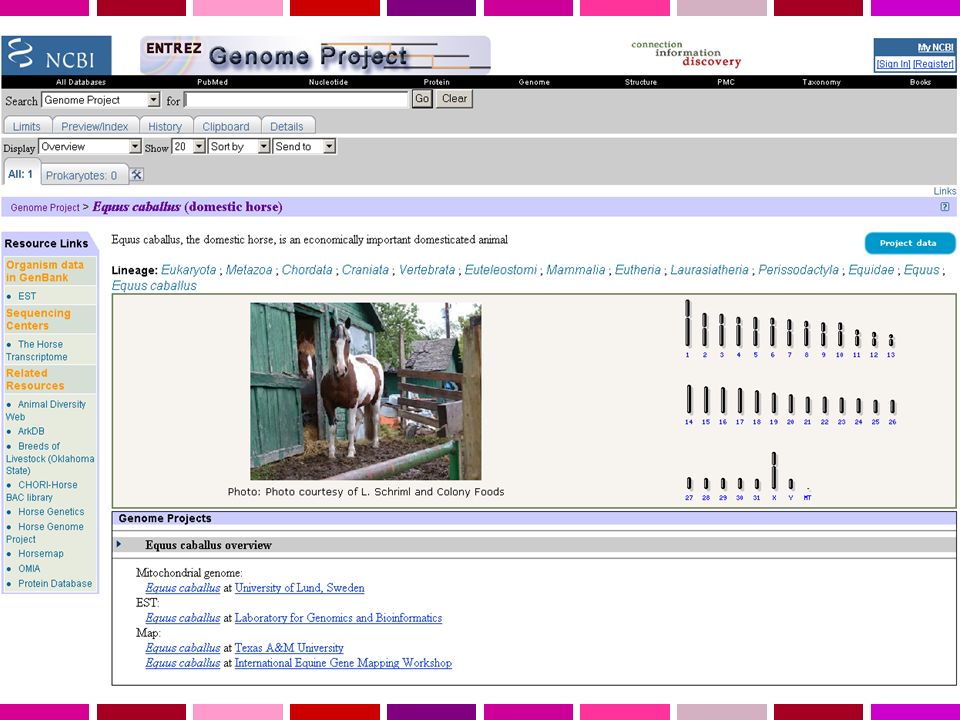
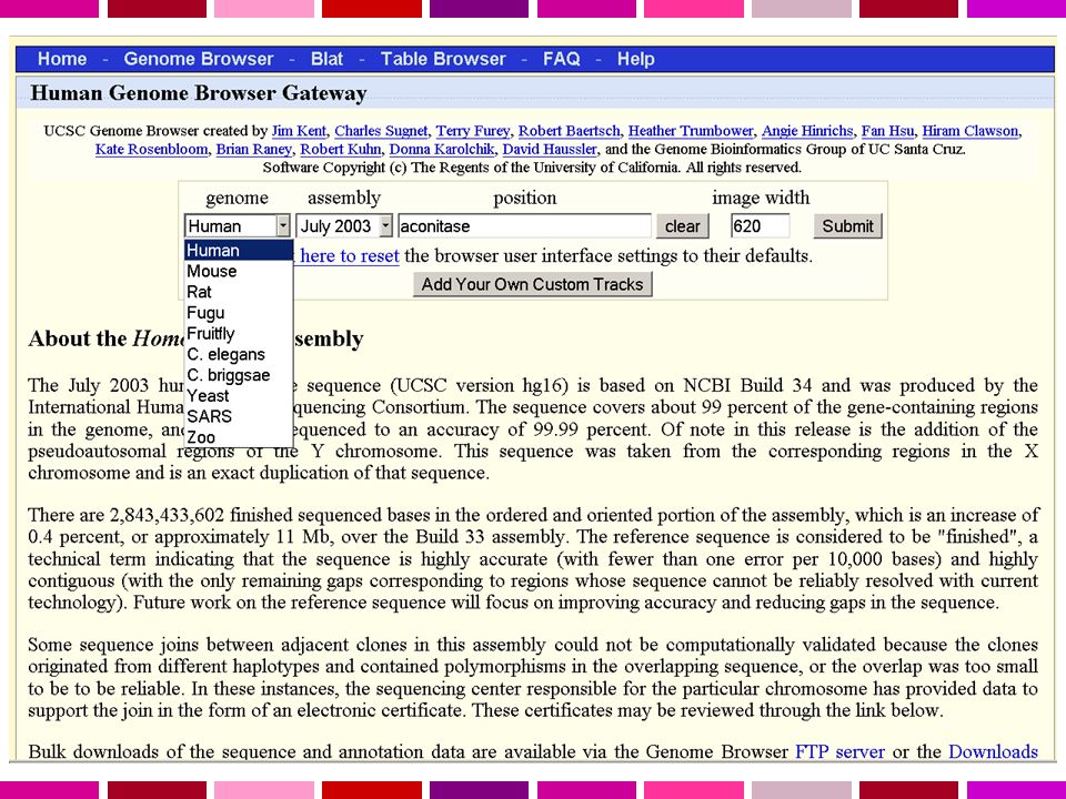
Servono: Annotazione dell’informazione sulla sequenza Possibilita’ di recuperare velocemente la sequenza di regioni specifiche del genoma in base a criteri di Contenuto di informazione Caratteristiche di sequenza Genomi disponibili Human Homo sapiens assembly 99% delle regioni contenenti geni accuratezza 99.99% 2.84 Gb finite “highly contiguous” Species A. gambiae A. mellifera C. briggsae C. elegans C. intestinalis Chicken Chimp Cow D. ananassae D. erecta D. grimshawi D. melanogaster D. mojavensis D. persimilis D. pseudoobscura D. sechellia D. simulans D. virilis UCSC Genome Browser Sistema per la “navigazione” della sequenza e dell’annotazione di genomi, che permette la visualizzazione dell’informazione a “diverso ingrandimento” ed il recupero di porzioni di sequenza con associate le informazioni di annotazione, come: Geni noti e geni predetti ESTs, mRNAs Isole CpG assembly gaps e coverage, bande cromosomiche Omologia con altri genomi … D. yakuba Dog Fugu Human Mouse Opossum Rat Rhesus S. purpuratus SARS Tetraodon X. tropicalis Yeast Zebrafish

14 UCSC Genome Browser Molte possibilita’ per la ricerca di una regione specifica: chr7 un cromosoma intero 20p13 una regione (banda p13 del cr. 20) chr3: il primo milione di basi del cr. 3 dal ptel D16S regione intorno al marcatore (100,000 basi per lato) RH18061;RH regione tra i due marcatori AA regione genomica che si allinea con la sequenza con questo GB accession number PRNP regione del genoma che comprende il gene PRNP NM_017414 NP_059110 (LLID) Oppure di liste di regioni: pseudogene mRNA Lists transcribed pseudogenes, but not cDNAs homeobox caudal Lists mRNAs for caudal homeobox genes zinc finger Lists many zinc finger mRNAs huntington Lists candidate genes associated with Huntington's disease

15

16

17

18 Overview of the whole Genome Browser page (mature release)
} Mapping and Sequencing Tracks Genes and Gene Prediction Tracks Genome viewer section Groups of data I wanted to just demonstrate an overview of a Genome Browser page at a mature stage of this assembly. You can see that there are many track and image controls seen down at the bottom of the page. At the very beginning of a release—there is only a CORE set of tracks at first, not all of the tracks are available. Over time these will be added to the browser—so the actual track options you see will accumulate over time. Tracks take time to create—within UCSC, and from other contributors all over the world. But I wanted to use this slide to illustrate one of the major organizational concepts of the Genome Browser. At the bottom of the page, you will find that the data is organized into GROUPS. These are groups of similar data, such as Mapping and Sequencing Tracks, Genes and Gene Prediction tracks, and so on. Each GROUP contains the individual TRACKS, or the lines of annotation. A group at the bottom of the page corresponds to a section in the viewer. In the viewer the separate GROUPs are indicated by the color change along the left side of the image area, from gray to blue and so on. Understanding this Group and Track organization will also help you to understand the Table Browser functions later. mRNA and EST Tracks Expression and Regulation Comparative Genomics ENCODE Tracks Variation and Repeats

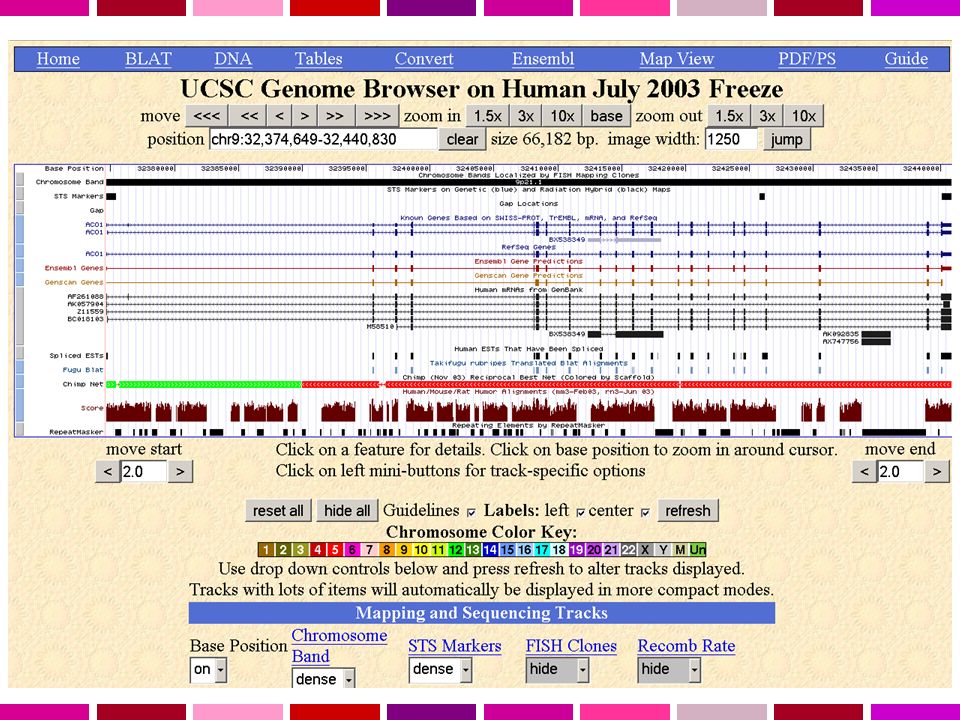
19 Sample Genome Viewer image, BRCA1 region
Genome backbone STS markers Known genes RefSeq genes Gene predictions GenBank mRNAs repeats GenBank ESTs conservation SNPs MGC clones At this time, I would like to focus on the viewer section of the Genome Browser. This is the default view, after a search for BRCA1. I wanted to quickly orient you to the things that you are seeing when you look at the default setup of the genome viewer. One of the first things to notice is that we can see that we are in the position of the genome that we expected by looking at the label on the side of the known gene track, which indicates the BRCA1 gene location—which I have highlighted in RED. At the very top of the image there is a track called BASE POSITION, which I have been calling the genome backbone. This is the actual base number of every single piece of the genome backbone. As you can see, were are around base number 38 million something-something-something…. As you look down the viewer, you will see many different data types are represented…STS markers, known genes, gene predictions, mRNAs, ESTs, evolutionary relationships, and repeats. This is just the default view, though—other data types are available for you to display. But what you can see right away is that you have a great deal of context about the BRCA1 position in the human genome.

20 Annotation Track options, defined
Hide: removes a track from view Dense: all items collapsed into a single line Squish: each item = separate line, but 50% height + packed Pack: each item separate, but efficiently stacked (full height) This slide just quickly defines the choices from the pulldown menus. You don’t need to memorize these—you can always refer back to the documentation or a Quick Reference Card for a refresher. But quickly, here are the choices, with some sample images of the same track and region with the different options: Hide: completely removes a track from your image Dense: all items become collapsed into a single line—fuses all the rows of data into one. Squish: each item is on a separate line, but at 50% of its regular height. Pack: each item is separate, but efficiently stacked like sardines. However, they are full height—which makes it different from squish. Full: each item is on a separate line. To choose any of these options, just highlight it in the pulldown menu. To make the changes happen, you have to click the REFRESH button that appears in the middle of the genome browser page. We’ll spend a little more time on the mid-page controls in a minute. Then we’ll move on to the last couple of features that you can use to adjust the images. Next slide. Full: each item on separate line

21 Clicking an annotation line, new page of detailed information
You will get detail for that single item you click Example: click on the BRCA1 Black “Known Genes” line New web page opens Many details and links to more data about BRCA1 Click the line Here I’ve just shown the small area of the annotation track image that I clicked, and a screen shot of the web page that you get from this click event. As you can see, the new web page says that you are looking at the detail for a KNOWN GENE [red box] It also gives you links out to other databases where you can learn more about this specific sequence—NCBI, PDB, SwissProt, OMIM, PubMed, mouse orthologs, and so on. We’ll take a closer look at that page in the next slide. The point is that one click away—on any item in the Genome Viewer--there is a LOT of more information available to you. One note: sometimes, if you click on an annotation track that is actually a compressed track, instead of going to a new web page the track will spread out. You have to click a second time to see the new web page in cases like that.

22 Click annotation track = BRCA1 “Known gene” detail page
informative description other resource links Not all genes have This much detail. Different annotation tracks carry different detail data. links to sequences microarray data mRNA secondary structure SNP detail page sample protein domains/structure As I showed on the previous slide, one level down there are information pages that contain LOTS of extra information about that gene (or predicted gene, or SNP, or other item) in the viewer. I’m going to just show one sample here of the detailed information on the human BRCA1 known gene page. But the other types of data also have lots of additional information one layer down as well. This page is actually quite huge, and I know that you won’t be able to see all the details right now. But later you should go and see for yourself. There is extensive information about this gene, and links to many other resources as well. Practially one-stop shopping for known genes! One thing to know: not all gene will have this level of detail, and not every species will have all this information. Some genes won’t have protein structures, some won’t have pathway information. But if the data is available, it will be available to you on these detail pages. I attached here a small part of a SNP detail page—position, sequence, validation status, function….and so on. Different data types will have different details pages. You just have to click on the item in the viewer to get to these details pages. homologs in other species Gene Ontology™ descriptions mRNA descriptions pathways

23 Getting the sequences Get DNA, with Extended Options; or Details pages
Use the DNA link at the top Plain or Extended options Change colors, fonts, etc. So—we have seen visual cues, and lots of text-based data. But one Frequently Asked Question that people have is “where is the sequence”? So I just want to spend a couple of slides on that topic so that you will know that you can get to the sequence level data. As I mention here, there are 2 handy ways to get the sequence information. First, from your BRCA1 viewer, you could simply click the link in the blue navigation bar at the top of the page [red box]. The link that says DNA will bring you to a new GET DNA web page, shown in the center. As you can see, the position you were looking at is specified. And on this page you have a bunch of options to format the sequence. --You can tweak the output by adding some bases on either side. --You can get the sequence in upper or lower case. --You can mask repeated, low complexity regions. --Or you can get the other strand. Just click the GET DNA button [red box] to get the sequence in a new web page, like I’ve shown here. The second option is the same in the beginning, but you can do even more to customize the output DNA. If you click the EXTENDED CASE/COLOR OPTIONS button, you’ll get a new page that lets you change the case of individual items, change their colors, underline specific things, and so on. The choices that you will see in the list are based on the things actively shown in the Genome Viewer window you were looking at. If that’s too much, go back and turn off some tracks….This is a really cool way to look at your sequence of interest! As you can see in a sample output, different features look different by color, case, or underlines. These two options that I just describe deal with getting the whole region of DNA from your viewer. But you have a 3rd option—you can get just the part you want from an annotation track; that’s what we’ll look at in the next slide.

24 Accessing the BLAT tool
In the UCSC browser, the tool you will use for sequence searching is called BLAT. Many of you will be familiar with the alignment tool called BLAST® or BLAST2, which stands for BASIC LOCAL ALIGNMENT SEARCH TOOL. {I swear I found the ® at ncbi: If you have used the NCBI databases, and searched for similar sequences, you have probably used BLAST. But BLAT is different—it is the Blast-like alignment tool. It goes about searching the database slightly differently than BLAST. But in the end you will have a pair of sequences that are lined up next to each other so you can compare the matches. Blat is really really fast—it has been optimized to search the whole genomes more quickly than BLAST does. For those people who care about this, it’s because the UCSC folks have created an INDEX of all the unique 11mers if it’s DNA, 4mers if protein (or stretches of 11nucleotides or 4 amino acids). Then when you throw a query sequence at it, it just looks down its index of 11mers, finds a match and works out from there. Blast does it the other way—it indexes your query and then runs your smaller index over everything…that’s the essential difference in the algorithm. It works best with sequences with high identity—but don’t let that scare you, you can find more distant matches as well. Directly from the UCSC documentation: “On DNA queries, BLAT is designed to quickly find sequences with 95% or greater similarity of length 40 bases or more. It may miss genomic sequences that are more divergent or shorter than these minimums, although it will find perfect sequence matches of 33 bases and sometimes as few as 22 bases. The tool is capable of aligning sequences that contain large introns. On protein queries, BLAT rapidly locates genomic sequences with 80% or greater similarity of length 20 amino acids or more. In general, gene family members that arose within the last 350 million years can generally be detected.” But for you algorithm hounds, you will realize that what I have said is really a simplification of the detailed algorithm, and I encourage you to investigate the details between the two methods by reading the papers for these. BLAST (original paper): Altschul SF, Gish W, Miller W, Myers EW, Lipman DJ. Basic local alignment search tool. J Mol Biol Oct 5;215(3): BLAT (original paper): W. James Kent (2002) BLAT - The BLAST-Like Alignment Tool, Genome Res 12: And for the more casual BLAT user, check out the documentation at the UCSC web site for a little more detail about the way BLAT works without tremendous amounts of mathematical equations…. For many people it will be enough to know that there is a means of searching for your region of interest in the database by starting with a sequence! So we’ll talk about how to use a sequence to get where you want now, using the BLAT software. Okay, so now we know a little bit about the BLAT tool. How do we get to it? Let’s start at the UCSC Genome Browser homepage, as I have shown here. There are a couple of ways, like we’ve seen before. You can use the Navigation bars at the top or at the side of the UCSC home page. Select the links called BLAT or BLAT search to get started. These will bring you to a BLAT web page, as shown in the next slide. BLAT = BLAST-like Alignment Tool Rapid searches by INDEXING the entire genome Works best with high similarity matches

25 BLAT tool overview: www.openhelix.com/sampleseqs.html
Make choices DNA limit bases Protein limit aa 25 total sequences Paste one or more sequences Here is the starting page for using BLAT to search the genomes at the UCSC browser. As you can see along the top there are a few parameters you can change—some choices you have to make. [red box 1] First, you must choose 1 species to search. Then you choose an assembly. Next, you may let the BLAT tool guess whether you have entered nucleotides or amino acids, or you can tell it which one you are using. Sort output—on default settings here—will list the best scoring matches first. Output type specifies whether you want the output to be in the browser form, or in files you can use later. Hyperlink is the default which displays in the browser, and that’s what I’ll be using for this example. There is a big text box where you can paste your sequence. [red box 2] You can paste 1 or more sequences, but there are limits to how much BLAT you can do, as it is a large burden on the servers. I have displayed 2 partial sequences here that I will use in my example. These are in the FASTA format, which you have to use if you are going to use multiple sequences. And there is also an option to upload your sequence (or sequences). [red box 3] Finally, you click SUBMIT to send your query to the database. There is a special new button—the “I’m Feeling Lucky” button. If you click that—just like in Google—you will be taken to the position of your best match right away, in the Genome Viewer. But I’ll be demonstrating the plain old SUBMIT button right now. Or upload Submit

26 BLAT results, with links
sorting Here we see the results of a BLAT search against the human genome, using the sample human mRNA sequences I showed. As you can see, we have sorted the list by the query and score [long red boxes ]. You can see we have a really really high scoring match up at the top. After that they appear to be less good matches—pretty small regions, probably. Now, you’ll remember that we asked for hyperlinked results, right? You can see that there are 2 columns of links for us. One says BROWSER, one says DETAILS. The first thing that I would do is click the BROWSER link for the matches [red box 2]. This will link me to the position of this match in the Genome Viewer. I will show a sample of that on the next slide. Later we will click on the DETAILS link for the best match. That will give us a new page with sequence information, as you’ll see a couple of slides from now. Results with demo sequences, settings default; sort = Query, Score Score is a count of matches—higher number, better match Click browser to go to Genome Browser image location (next slide) Click details to see the alignment to genomic sequence (2nd slide)

27 BLAT results, alignment details browser
Click to flip frame Watch out for reading frame! Click > to flip frame Base position = full and zoomed in enough to see amino acids query matches From browser click in BLAT results A new line with your Sequence from BLAT Search appears! When you link from the BLAT results to the BROWSER—you get a special track! Just down from the top there is a new line on the browser—it says YOUR SEQUENCE FROM BLAT SEARCH. And the name of my query sequence is listed over on the left…. And if you look at the known genes, or refseq genes, you can see that we have matched the CXCL5 gene, which is what we would have expected from the BLAT query. On the known genes, you can see the Methionines indicated in green. Also, note the direction of this gene—it is on the negative strand, therefore runs from right to left in this case. But beware—the 3 frame translation at the top is running the other way. If you want to compare the methionines, you have to flip the frame translation. So—we have used a sequence as a starting point to search the genome. We get to see the actual alignment data, and we get to see the location of our match on the Genome Browser. So BLAT is another good place to start searching for your genes of interest in the UCSC Genome Browser tool. One special tip here: when you are zoomed in enough on a sequence, you can see the amino acids in the display. But be careful of the reading frame direction—check your known gene arrowheads. If you have to flip the frame—because the default is the 3 frames in the 5’ to 3’ direction, click the small arrow underneath BASE POSITION to flip the nucleotide or amino acid direction.

28 BLAT results, alignment details
Your query Genomic match, color cues Side-by-side alignment Here I show the outcome if you clicked the DETAILS link from the BLAT results page. I know it’s impossible to see the whole alignment page—even with my tiny little query sequence this is a really big web page that you get. You can see the page is divided into several parts. The top part shows the query sequence you put in (in this case our human CXCL5 DNA sequence). The middle part of the page shows the match up of your sequence (in blue) capital letters, to the genomic sequence. This gives you a really quick look at the exon/intron structure—right? It’s a nice way to see which parts are the exons in an mRNA (if that’s what you started with), and the introns in black text. The bottom part shows you the actual nucleotide-for-nucleotide matches—this may be more like the BLAST results you are used to seeing. I magnified the top of the side-by-side alignment so you can see where my query sequence on the top (starts with number ), lines up with the genomic sequence. You can judge the quality of the match yourself in this section. Okay—I’m convinced that this sequence matched up perfectly with the genomic sequence, and that’s the region I want to examine in the genome browser. So, if you use the back button on your browser to get back to your results list, you can now select the other link to go directly to the genome viewer for this match region.