I e la loro previsione parte seconda

I e la loro previsione parte seconda
TERREMOTI Prof. Roberto Scarpa Ordinario di Fisica Terrestre Direttore Centro Interdipartimentale di Scienze Ambientali Università di Salerno

Magnitude 9.0 NEAR THE EAST COAST OF HONSHU, JAPAN Friday, March 11, 2011 at 05:46:23 UTC
Japan was struck by a magnitude 9.0 earthquake off its northeastern coast Friday. This is one of the largest earthquakes that Japan has ever experienced. . In downtown Tokyo, large buildings shook violently and there is severe flooding due to a tsunami generated by the earthquake. USGS Part of houses swallowed by tsunami burn in Sendai, Miyagi Prefecture (state) after Japan was struck by a strong earthquake off its northeastern coast Friday, March 11, 2011. New York Times

Tsunami waves swept away houses and cars in northern Japan and pushed ships aground. The tsunami waves traveled far inland, the wave of debris racing across the farmland, carrying boats and houses with it. The tsunami, seen crashing into homes in Natori, Miyagi prefecture. AP Houses were washed away by tsunami in Sendai, Miyagi Prefecture in eastern Japan, after Japan was struck by a magnitude 9.0 earthquake off the northeastern coast. New York Times

CNN reported “The quake rattled buildings and toppled cars off bridges and into waters underneath. Waves of debris flowed like lava across farmland, pushing boats, houses and trailers toward highways.” Additionally, a number of fires broke out including one at an oil refinery which at this time, is burning out of control. Giant fireballs rise from a burning oil refinery in Ichihara, Chiba Prefecture (state) after Japan was struck by a strong earthquake off its northeastern coast Friday, March 11, 2011. Los Angeles Times

This earthquake occurred 130 km (80 miles) east of Sendai, Honshu, Japan and 373 km (231 miles) northeast of Tokyo, Japan. Images courtesy of the US Geological Survey

Shaking intensity scales were developed to standardize the measurements and ease comparison of different earthquakes. The Modified-Mercalli Intensity scale is a twelve-stage scale, numbered from I to XII. The lower numbers represent imperceptible shaking levels, XII represents total destruction. A value of IV indicates a level of shaking that is felt by most people. Perceived Shaking Extreme Violent Severe Very Strong Strong Moderate Light Weak Not Felt Modified Mercalli Intensity Image courtesy of the US Geological Survey USGS Estimated shaking Intensity from M 9.0 Earthquake

USGS PAGER Population Exposed to Earthquake Shaking The USGS PAGER map shows the population exposed to different Modified Mercalli Intensity (MMI) levels. MMI describes the severity of an earthquake in terms of its effect on humans and structures and is a rough measure of the amount of shaking at a given location. Overall, the population in this region resides in structures that are resistant to earthquake shaking. The color coded contour lines outline regions of MMI intensity. The total population exposure to a given MMI value is obtained by summing the population between the contour lines. The estimated population exposure to each MMI Intensity is shown in the table below. Image courtesy of the US Geological Survey

Globally, this is the 4th largest earthquake since 1900.
Magnitude 9.0 NEAR THE EAST COAST OF HONSHU, JAPAN Friday, March 11, 2011 at 05:46:23 UTC Globally, this is the 4th largest earthquake since 1900. Chile 1960 Alaska 1964 Sumatra 2004 Russia 1952 Japan 2011 Ecuador 1906 Alaska 1965 Chile 2010

Peak ground acceleration is a measure of violence of earthquake ground shaking and an important input parameter for earthquake engineering. The force we are most experienced with is the force of gravity, which causes us to have weight. The peak ground acceleration contours on the map are labeled in percent (%) of g, the acceleration due to gravity. Map showing measured Peak Ground Accelerations across Japan measured in percent g (gravity). Image courtesy of the US Geological Survey

Earthquake and Historical Seismicity
Magnitude 9.0 NEAR THE EAST COAST OF HONSHU, JAPAN Friday, March 11, 2011 at 05:46:23 UTC Earthquake and Historical Seismicity This earthquake (gold star), plotted with regional seismicity since 1990, occurred at approximately the same location as the March 9, 2011 M 7.2 earthquake. In a cluster, the earthquake with the largest magnitude is called the main shock; anything before it is a foreshock and anything after it is an aftershock. A main shock will be redefined as a foreshock if a subsequent event has a larger magnitude. This earthquake redefines the M 7.2 earthquake as a foreshock, with this event replacing it as the main shock. Image courtesy of the US Geological Survey

This earthquake was the result of thrust faulting along or near the convergent plate boundary where the Pacific Plate subducts beneath Japan. This map also shows the rate and direction of motion of the Pacific Plate with respect to the Eurasian Plate near the Japan Trench. The rate of convergence at this plate boundary is about 83 mm/yr (8 cm/year). This is a fairly high convergence rate and this subduction zone is very seismically active. Japan Trench

The map on the right shows historic earthquake activity near the epicenter (star) from 1990 to present. As shown on the cross section, earthquakes are shallow (orange dots) at the Japan Trench and increase to 300 km depth (blue dots) towards the west as the Pacific Plate dives deeper beneath Japan. Seismicity Cross Section across the subduction zone showing the relationship between color and earthquake depth. Images courtesy of the US Geological Survey

At the latitude of this earthquake, the Pacific plate moves approximately westwards with respect to the Eurasian plate at a velocity of 83 mm/yr. The Pacific plate thrusts underneath Japan at the Japan Trench, and dips to the west beneath Eurasia. The location, depth, and focal mechanism of the March 11 earthquake are consistent with the event having occurred as thrust faulting associated with subduction along this plate boundary. Shaded areas show quadrants of the focal sphere in which the P-wave first-motions are away from the source, and unshaded areas show quadrants in which the P-wave first-motions are toward the source. The dots represent the axis of maximum compressional strain (in black, called the "P-axis") and the axis of maximum extensional strain (in white, called the "T-axis") resulting from the earthquake. USGS Centroid Moment Tensor Solution

Large earthquakes involve slip on a fault surface that is progressive in both space and time. This “map” of the slip on the fault surface of the M 9.0 Japan earthquake shows how fault displacement propagated outward from an initial point (or focus) about 24 km beneath the Earth’s surface. The rupture extended over 500 km along the length of the fault, and from the Earth’s surface to depths of over 50 km. Image courtesy of the U.S. Geological Survey Cross-section of slip distribution. The strike direction of the fault plane is indicated by the black arrow and the hypocenter location is denoted by the red star. The slip amplitude are showed in color and motion direction of the hanging wall relative to the footwall is indicated by black arrows. Contours show the rupture initiation time in seconds.

Although magnitude is still an important measure of the size of an earthquake, particularly for public consumption, seismic moment is a more physically meaningful measure of earthquake size. Seismic moment is proportional to the product of the slip on the fault and the area of the fault that slips. This graph of the moment rate function describes the rate of moment release with time after earthquake origin. The largest amounts of rupture occurred over 100 seconds but smaller displacements continued for another 75 seconds after the start of the earthquake. Image courtesy of the U.S. Geological Survey

The moment magnitude scale is designed to give an accurate characterization of the true size of an earthquake, but be tied to the original description of magnitude that was developed by Charles Richter. Moment magnitude accounts for earthquake size by looking at all the energy released. It is striking that only 6 earthquakes over the last 106 years account for over half of the energy released during that time. New Mexico Institute of Mining and Technology

This earthquake was preceded by a series of large foreshocks over the previous two days, beginning on March 9th with an M 7.2 event approximately 40 km from the March 11 earthquake, and continuing with 3 earthquakes greater than M 6 on the same day. The M 9.0 earthquake has been followed by frequent large aftershocks, which can do damage on their own especially to buildings that were compromised in the main shock. The M 9.0 main shock (red star) is plotted with 14 aftershocks larger than magnitude 6.0 that occurred in the first 6 hours after the earthquake. This includes a magnitude 7.1.

Aftershocks Aftershock sequences follow predictable patterns as a group, although the individual earthquakes are themselves not predictable. The graph below shows how the number of aftershocks and the magnitude of aftershocks decay with increasing time since the main shock. The number of aftershocks also decreases with distance from the main shock. Aftershocks usually occur geographically near the main shock. The stress on the main shock's fault changes drastically during the main shock and that fault produces most of the aftershocks. Sometimes the change in stress caused by the main shock is great enough to trigger aftershocks on other, nearby faults. Image and text courtesy of the US Geological Survey

Seismic waves recorded around the world.
Magnitude 9.0 NEAR THE EAST COAST OF HONSHU, JAPAN Friday, March 11, 2011 at 05:46:23 UTC Seismic waves recorded around the world.

Preannunciare i terremoti
In inglese vengono utilizzati due differenti termini che in italiano sono quasi sinonimi (forecasting e prediction), e possono essere tradotti come previsione e predizione. Il preannuncio o previsione (forecasting) è meno preciso Basato sui periodi di ritorno dei terremoti piuttosto che sulla identificazione di segnali premonitori Le faglie attive o i segmenti di faglia non si fratturano in modo caotico Hanno periodi di ritorno caratteristici Riflettono accumulo di deformazione lungo la faglia e la capacità di una faglia a resistere fino ad un valore caratteristico per quell’assegnata faglia o parte di essa Esistono ulteriori complicazioni: La frattura non avviene secondo un tempo ben delimitato, ma piuttosto esiste un’intervallo abbastanza ampio di periodi di ritorno, corrispondente alle incertezze con cui conosciamo le condizioni al contorno del problema La deformazione può avvenire mediante un grande terremoto o una serie di eventi di dimensioni più moderate(e.g. Marmara Sea a sud di Istanbul) Tutto ciò ha enormi implicazioni per la stima del rischio sismico

L’esempio della faglia di San Andreas
Prima del terremoto di San Francisco del 1906 ( M=8.25) ~ 3.2m spostamento lungo la faglia in 50 anni. La deformazione associata al terremoto fu ~ 6.5m Tempo necessario per l’accumulo di sforzi (6.5/3.2) x 50 ~100 anni Periodo di ritorno fino al prossimo terremoto di grandezza confrontabile = 100 anni Tutto ciò assumendo: Accumulo uniforme di deformazione Il terremoto non altera le proprietà del mezzo

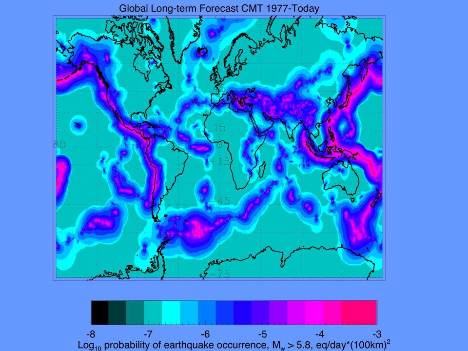
Problemi con le previsioni a lungo termine
Tali previsioni sono affidabili solo per i cataloghi più attendibili I cataloghi storici sono soddisfacenti solo per alcune regioni come la California, Giappone, Europa, Cina Insoddisfacenti per le regioni con sismicità a bassa frequenza ma di elevate magnitudo Zona di subduzione Cascadia New Madrid Giamaica Europa occidentale I cataloghi hanno bisogno di essere integrati con studi paleosismologici Zona di subduzione Cascadia

La teoria delle lacune (gap sismici)
La lacuna o gap sismico è definita come una regione sismica dove c’è stato un rilascio di energia stto il livello normale di attività. Il terremoto di Loma Prieta del 1989 riempì una lacuna, asismica fin dal 1906 Altre lacune esistono in: Arco Aleutino (Alaska) Istanbul Tokai (Giappone) California meridionale La lacuna di Istanbul

27/03/2017

Lacuna sismica dell’evento di Loma Prieta 1989 (M 7.1)

Definizione delle lacune sismiche nel Mediterraneo (1979)

Previsione dell’intensità sismica
Altri utili parametri possono essere predetti al posto del tempo. Prevedere l’intensità sismica in un’area è particolarmente utile per: Pianificazione di strutture come dighe, scuole, ospedali e centri di emergenza; Costruzione di mappe di rischio E’ richiesta una dettagliata conoscenza della geologia e della risposta sismica locale. Previsione dell’intensità attesa nella regione del Tokai, Giappone

Previsione probabilistica
Il più utile e corretto modo per esprimere la previsione di un futuro terremoto viene effettuata in termini probabiistici La maggioranza delle persone dovrebbe essere familiare con le probabilità a causa della diffusione del gioco d’azzardo Esempio nella regione di San Francisco (Bolt, 1999) 5 terremoti > M = 6.75 in 155 anni tra 1836 & 1991 Se gli eventi sono casuali, un altro evento  6.75 può essere atteso in 155/5 anni = 31 anni con elevata probabilità Problema: I terremoti non sono completamente casuali. Su di un assegnato sistema di faglie I terremoti sono raggruppati (a causa del trasferimento di sforzo) o seguono particolari andaenti spazio-temporali Un metodo alternativo per una previsione probabilistica si basa sul modello del rimbalzo elastico Questo si basa su stime dell’accumulo di sforzi sulla faglia

Misura della deformazione e previsione
Mappe geologiche sono utilizzate per definire segmenti di faglia attivi Sono effettuate assunzioni sulla propagazione della rottura di assegnati segmenti Poichè la deformazione si lega alla magnitudo, per una assegnata lunghezza di segmenti, ciò fornisce il terremoto massimo atteso La relazione tra Ms e la lunghezza della frattura L: M s = log L

Calcolo delle probabilità
Si determina la storia dello scorrimento su ciascun segmento di faglia Si calcola la velocità di accumulo della deformazione per ciascun segmento La storia dello scorrimento per ciascun segmento di faglia è rappresentata in funzione del tempo Poichè lo scorrimento è legato alla magnitudo, ciò permette di determinare gli intervalli di ricorrenza tra terremoti maggiori di valori assegnati di magnitudo Scorri- mento Tempo Magnitudo 6

Istogramma delle probabilità di un terremoto
Frequenza sismica Tempo di ricorrenza T1 T2 Si costruisce un istogramma che mostra in N. di terremoti che avvengono in uno specifico periodo di ricorrenza L’intervallo di ricorrenza più probabile è quello che divide l’istogramma in due parti eguali. Se il tempo dall’ultimo terremoto di un’assegnata magnitudo è T1, la probabilità del prossimo terremoti in T1 - T2 anni = rapporto dell’area rossa rispetto a quela gialla Man mano che il tempo di ricorrenza T2 cresce, tale rapporto si avvicina a 1 ed il terremoto diventa virtualmente certo Più è stimato in modo preciso il tempo di ricorrenza e migliore è la previsione statistica

L’istogramma della probabilità di terremoto e la faglia San Andreas
La California e il sistema di faglie di San Andreas sono particolarmente adatti per la loro esposizione in superficie. Permette di misurare facilmente gli spostamente e di monitorare la deformazione Il metodo dipende in modo cruciale dalla stima dei potenziale teremoti distruttivi in tempi storici e dalla loro datazione Il problema è approfonditamente discusso nel libro di Bolt (1999) p )

Carte delle probabilità di eventi con magnitudo>6
Carte delle probabilità di eventi con magnitudo>6.7 nella regione di San Francisco ( ) Cart

Predire i terremoti Capitolo estremamente controverso della Sismologia
Implica un allarme preciso sul tempo e la grandezza di un futuro terremoto Si basa sull’occorrenza di chiari segnali premonitori di un terremoto Il metodo deve essere rigoroso e ripetibile per un suo efficace utilizzo In una zona di elevata sismicità, una qualsiasi predizione ha una probabilità>0 di essere corretta In ogni caso una predizione non corretta implica che il metodo o la teoria sono errati

Precursori sismici Cambiamenti nelle velocità crostali delle onde sismiche Deformazioni crostali Cambiamenti nelle acque sotterranee Rilascio di gas Effetti atmosferici Comportamento anomalo degli animali Cambiamenti nelle proprietà elettromagnetici delle rocce Il cosiddetto metodo VAN

Fenomenologia della teoria della dilatanza-diffusione (Scholz et al

La previsione mancata del 1985
23 gennaio 1985: per la prima (e unica) volta in Italia scatta l’allarme terremoto. L’Istituto Nazionale di Geofisica prevede una «scossa pericolosa ». E il ministro della Protezione civile Giuseppe Zamberletti, oggi presidente della Commissione grandi rischi e sostenitore dell’impossibilità di prevedere i terremoti, ordina lo stato d’allerta per dieci comuni della Garfagnana: scuole chiuse per due giorni, case vecchie o in cattivo stato evacuate. Centomila persone abbandonarono le proprie abitazioni, ma il terremoto non arrivò. Allora la previsione di un sisma distruttivo fu formulata, dopo una scossa premonitrice, sulla base di un’analisi storico-statistica. Nel 1985 la «scossa pericolosa» non arrivò. E l’ex ministro Zamberletti finì sotto inchiesta per procurato allarme. Forse per questo da allora ha sempre chiamato i centomila sfollati «un test». E oggi ribadisce: «I terremoti non sono prevedibili». Ma poi spiega: «Allora il radon non c’entrava, lì ci trovavamo davanti a dati statistici particolari. Davanti a una previsione della comunità scientifica come quella di 25 anni fa, proprio Boschi e Barberi mi avvertirono del rischio, farei la stessa cosa: ordinerei lo stato d’allerta».

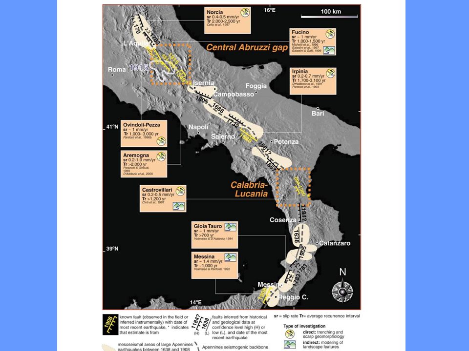
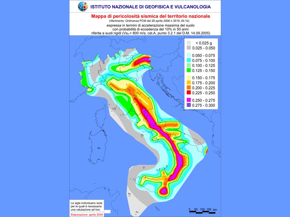
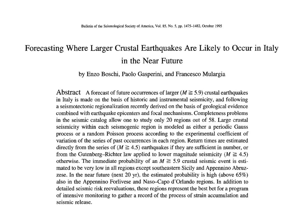
Zonazione sismica italiana ZS4

Mappa dei LNGS e UNDERSEIS

Terremoti italiani più catastrofici
Appennino centro-meridionale ( vittime) 1693 – Sicilia orientale ( vittime) 1688/1694/1703 – Appennino centro-meridionale ( vittime) 1783 – Calabria ( vittime) 1857 – Appennino meridionale ( vittime) 1908 – Sicilia ( vittime) 1915 – Appennino centrale ( vittime)

Terremoti più rilevanti (M≥6.5) del XX secolo
Calabria Ms=7.3 Messina Ms=7.0 Avezzano Ms=6.8 1930 – Irpinia Ms=6.5 1938 – Basso Tirreno mB=6.8 1976 – Friuli Ms=6.5 1980 – Campania-Lucania Ms=6.9

Ed il prossimo terremoto in Italia?
Le aree italiane a più elevato potenziale sismico sono alcune dell’appennino centro-meridionale (aquilano, beneventano) e dell’appennino calabro-siculo (Sicilia orientale, Calabria) quiescenti da circa 300 anni. In queste occorrerebbe potenziare le conoscenze e la divulgazione scientifica, oltre che il rafforzamento ed il controllo degli edifici.

Conclusioni Thomas Kuhn (La struttura delle rivoluzioni scientifiche, Einaudi, 1979) ha dibattuto in questo saggio come si possa distinguere tra predizioni di tipo scientifico e non scientifico. Come esempio egli ha confrontato l’astronomia con l’astrologia: entrambe effettuano delle predizioni che falliscono in diversi casi. Comunque gli astronomi imparano da questi errori, modificano ed aggiornano i loro modelli seguono il metodo scientifico Galileano mentre gli astrologi no.

I e la loro previsione parte seconda

Presentazioni simili

Presentazione sul tema: "I e la loro previsione parte seconda"— Transcript della presentazione:

Presentazioni simili

Sul progetto

Feed-back

Entrare

Autorizzarsi attraverso i social network:

I e la loro previsione parte seconda

Presentazioni simili

Presentazione sul tema: "I e la loro previsione parte seconda"— Transcript della presentazione:

Presentazioni simili

Sul progetto

Feed-back