Scaricare la presentazione
La presentazione è in caricamento. Aspetta per favore

1
Una veloce presentazione
Il Progetto PELCOM Una veloce presentazione (Silvio GRIGUOLO - DAEST/IUAV) Qualche slide iniziale è tratta da una presentazione di Sander Mucher, Wageningen, coordinatore del progetto Le ultime slides sull’applicazione alla biodiversità sono di Camiel Heunks, del National Institute for public Health and the Environment (RIVM) La presentazione usa sia l’italiano che l’inglese
 Qualche slide iniziale è tratta da una presentazione di. Sander Mucher, Wageningen, coordinatore del progetto. Le ultime slides sull’applicazione alla biodiversità sono. di Camiel Heunks, del National Institute for public. Health and the Environment (RIVM) La presentazione usa sia l’italiano che l’inglese.")
2
the PELCOM Project Land Cover Classification at the continental scale
A shared Cost Action, EU 4th framework Environment & Climate Start September ‘96 - End November ‘99

3
PELCOM Pan European Land COver Monitoring
(Research funded by the European Commission) Wageningen UR ( formerly DLO) Austrian Research Centre Seibersdorf (ARCS) Centre National de Recherches Meteorologiques (CNRM) - Toulouse National Institute for Public Health and the Environment (RIVM) Swedish Space Corporation (SSC) Instituto Universitario di Architettura (IUAV) Space Applications Institute (SAI-JRC) Geodan
 Wageningen UR ( formerly DLO) Austrian Research Centre Seibersdorf (ARCS) Centre National de Recherches Meteorologiques (CNRM) - Toulouse. National Institute for Public Health and the Environment (RIVM) Swedish Space Corporation (SSC) Instituto Universitario di Architettura (IUAV) Space Applications Institute (SAI-JRC) Geodan.")
4
PELCOM Homepage

5
Perché il Progetto PELCOM?

6
Stato dell’arte CORINE-LC procede a rilento
Altri database raster esistenti sono largamente basati su statistiche amministrative La classificazione DISCover (IGBP) ha un livello di dettaglio insufficiente per l’Europa Il progetto FIRS si concentra soprattutto sulle foreste
 ha un livello di dettaglio insufficiente per l’Europa. Il progetto FIRS si concentra soprattutto sulle foreste.")
7
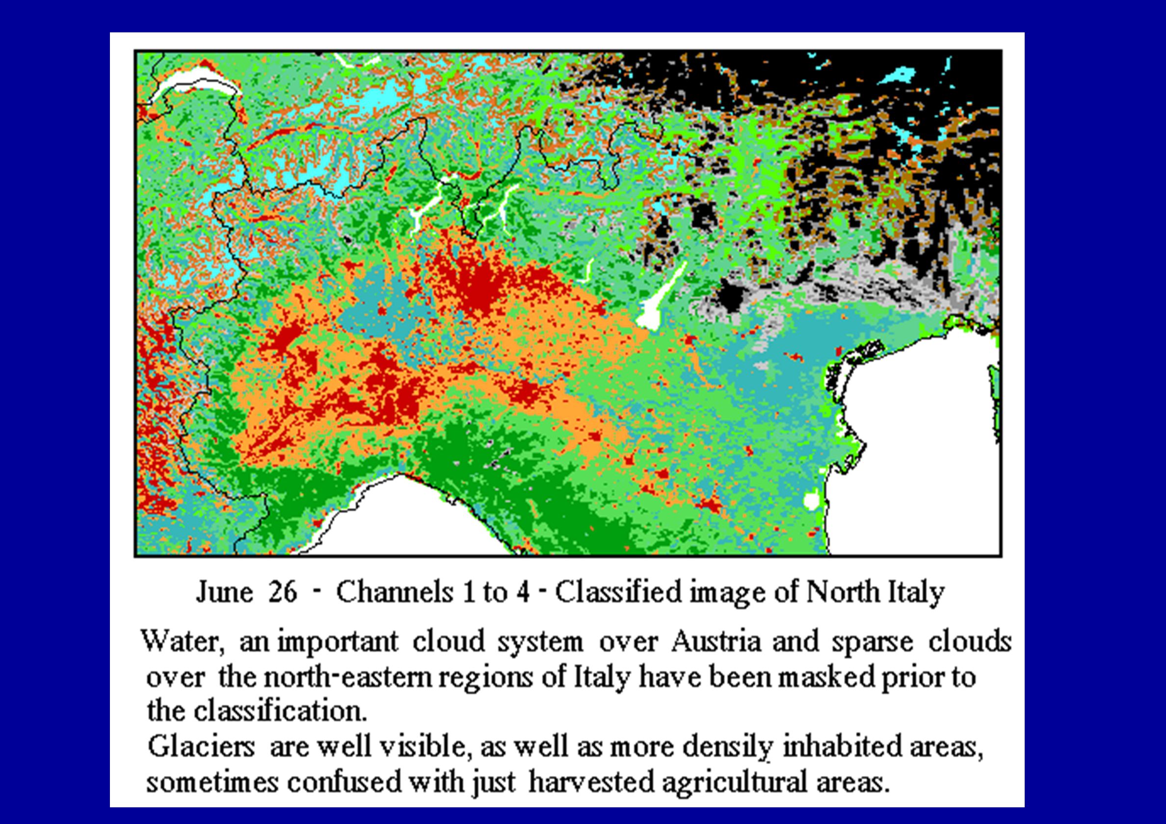
CORINE land cover database

8
Detail of IGBP global land cover database

9
Manca un’informazione aggiornata del Land Cover per l’intera Europa
In definitiva... Manca un’informazione aggiornata del Land Cover per l’intera Europa

10
Dunque… investigare l’applicabilità delle immagini satellitari NOAA-AVHRR per:
Mapping Monitoring

11
Gli obiettivi del Progetto
definizione di una metodologia di classificazione consistente Costruzione di una database raster delle coperture del suolo (Land Cover) ad 1 km dell’intera Europa, da utilizzare come input per modelli dinamici ambientali alla scala continentale Applicazioni sperimentali della mappa
 ad 1 km. dell’intera Europa, da utilizzare come. input per modelli dinamici ambientali alla. scala continentale. Applicazioni sperimentali della mappa.")
12
Fasi (1996-99) 1st year sviluppo della metodologia di
classificazione e monitoraggio 2nd year esperimenti regionali di classificazione 3rd year Studio di casi su ambiente & clima

13
Primi esperimenti di modellistica
Modello dinamico della bio-diversità, basato sulla definizione di Natural Capital Index (pressione sulla bio-diversità dovute a cambiamenti climatici, densità di insediamento umano, consumo e produzione, acidificazione, eutrofizzazione, ozono, ecc.)
")
14
RIVM - Indice di pressione sulla bio-diversità nelle aree naturali
(proiezione al 2010)
")
15
applicazione a modelli metereologici.
MeteoFrance (Toulouse): applicazione a modelli metereologici. Gli scambi vegetazione-atmosfera sono una componente importante nei modelli numerici di previsione del tempo. La mappa PELCOM della vegetazione è stata assunta come input per il modello metereolo- gico ARPEGE-ALADDIN.
: applicazione a modelli metereologici. Gli scambi vegetazione-atmosfera sono una. componente importante nei modelli numerici di. previsione del tempo. La mappa PELCOM della vegetazione è stata. assunta come input per il modello metereolo- gico ARPEGE-ALADDIN.")
16
VOC emission dalle foreste usando PELCOM (ARCS)
Le piante sono una delle maggiori fonti di Composti Organici Volatili, a loro volta precursori della formazione di ozono. L’emissione di composti organici è ritenuta una risposta fisiologica delle piante ai fattori di stree ambientale, come l’alta temperatura o la scarsità idrica.

17
I dati

18
Materiali AVHRR NDVI monthly MVC’s 1997
AVHRR Daily Multi-spectral mosaics ‘95/’96/’97 Ancillary geographic data: CORINE land cover data FIRS regions and strata Digital Chart of the World

19
Il Digital Terrain Model (raster) per la nostra area (1430x1700)
 per la nostra area (1430x1700)")
20
The digital Forest Map looks reasonable….

21
….yet some details are quite strange.

22
Regional approach - FIRS regions and strata
Regions in Colours Strata in Yellow lines Similar NDVI profiles may have a different meaning in different regions

23
Regional approach AOI per partner: Yellow: SSC Green: SC-DLO
Black lines FIRS regions Red lines FIRS strata AOI per partner: Yellow: SSC Green: SC-DLO Blue: CNRM Purple: ARCS Orange: IUAV Source: EMAP unit (SAI-JRC)
")
24
Defined Classification Methodology
Regions and strata Multi-spectral AVHRR data NDVI ‘97 Masks CORINE Pure Pixels Classification Masked NDVI Data base Compilation Enhancements Post-classification 1st - best 2nd - best classes Signatures Distances

25
PELCOM 1km land cover database
Conif. Forest Decid. Forest Mixed Forest Grassland Arable land Irrigated land Permanent crops Shrubland Barren land Ice and Snow Wetlands Water Urban

26
PELCOM land cover - Pixel: 1.1 km
![]()
27
Our Areas of Interest, each including one or more FIRS strata
Our Areas of Interest, each including one or more FIRS strata. The parts pointed at by arrows show where strata extend into regions for which no CORINE info exists.

28
IUAV - South-East Europe - Final classified image

29
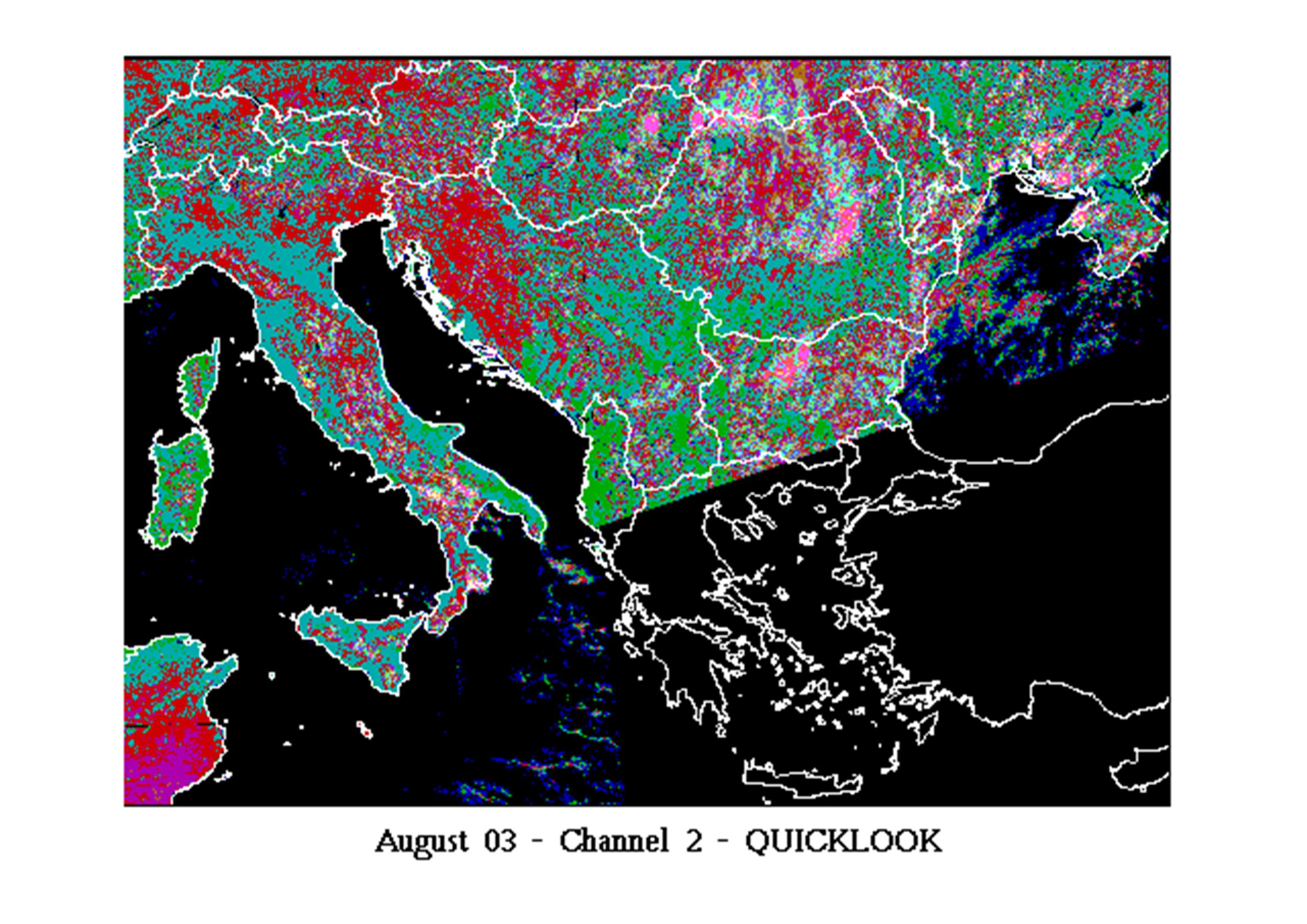
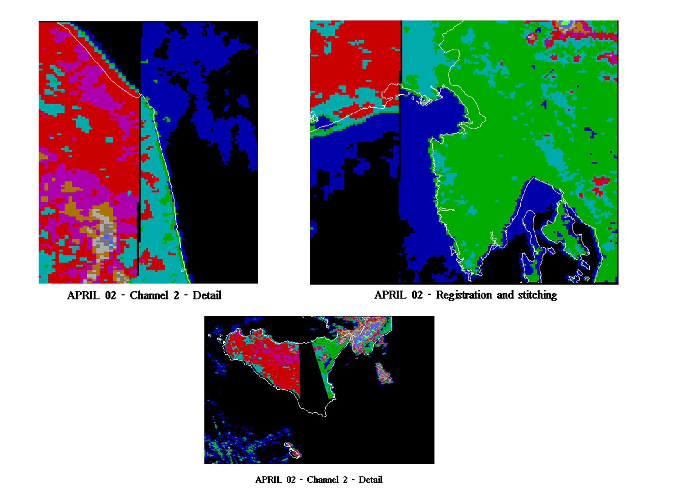
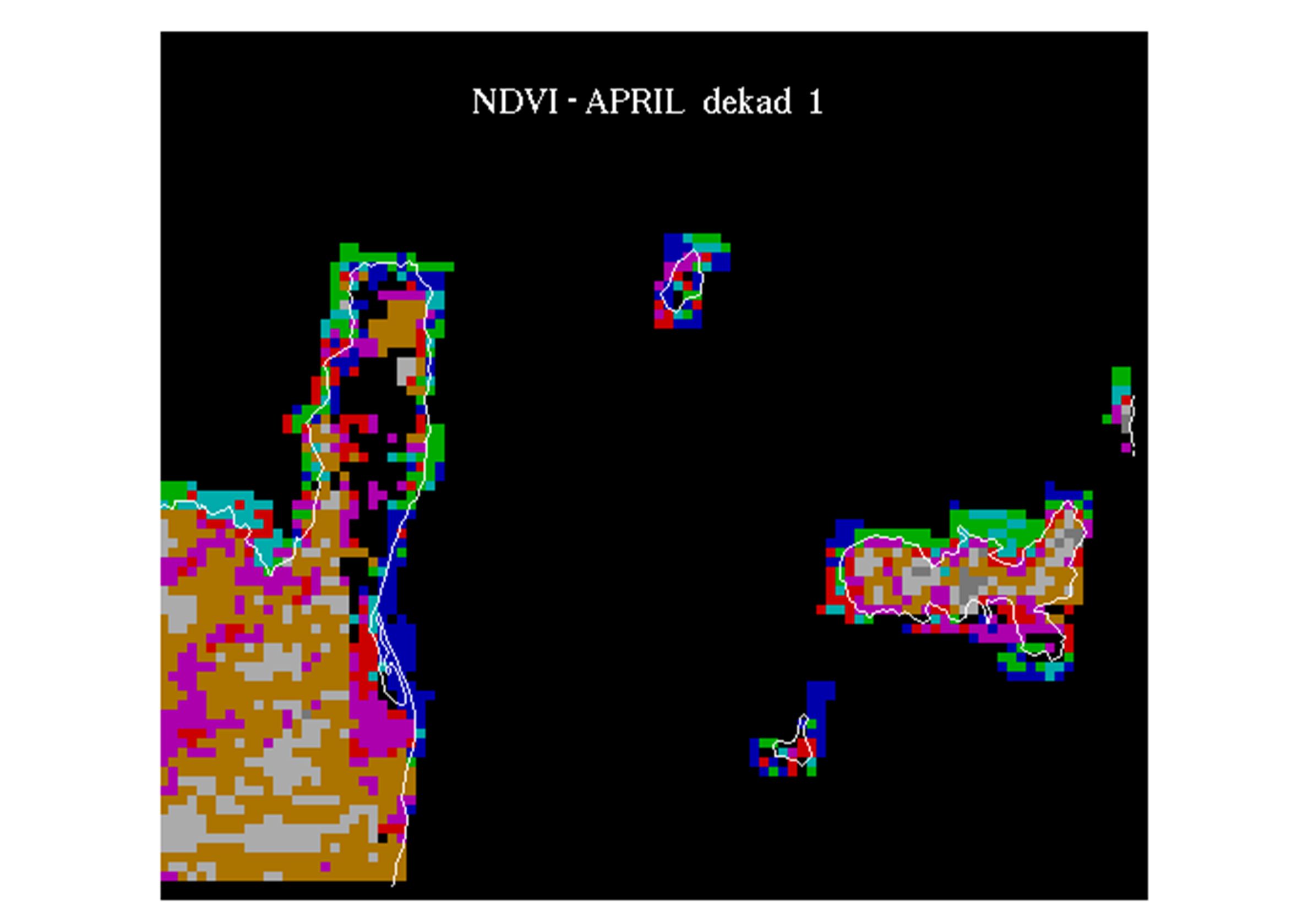
Scelta delle immagini e problemi connessi
Archivio MARS/JRC : immagini NOAA-AVHRR, 1995, multispettrali, diverse date; cattiva registrazione, nuvole Archivio MARS/JRC: immagini decadali NDVI, MVC Archivio MARS/JRC: immagini processate SMART problemi di registrazione Archivio EROS (IGBP) immagini 1995 migliori, ma forse è solo apparente DLR Berlino: MVC NDVI, mensili e decadali
 immagini migliori, ma forse è solo apparente. DLR Berlino: MVC NDVI, mensili e decadali.")
47
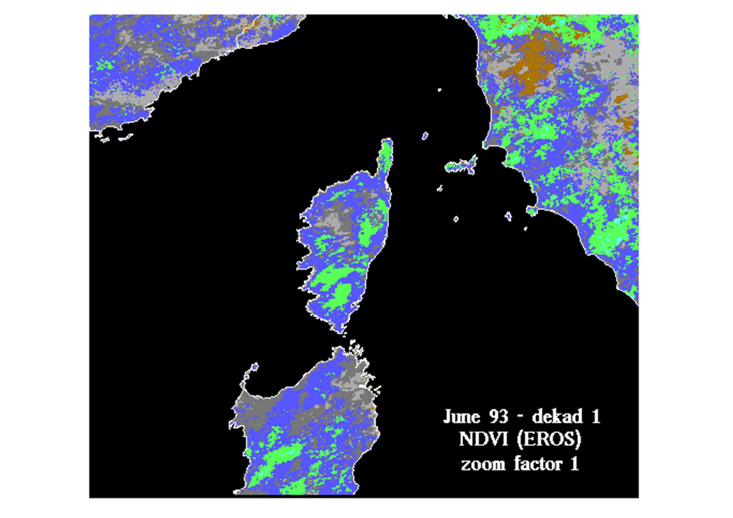
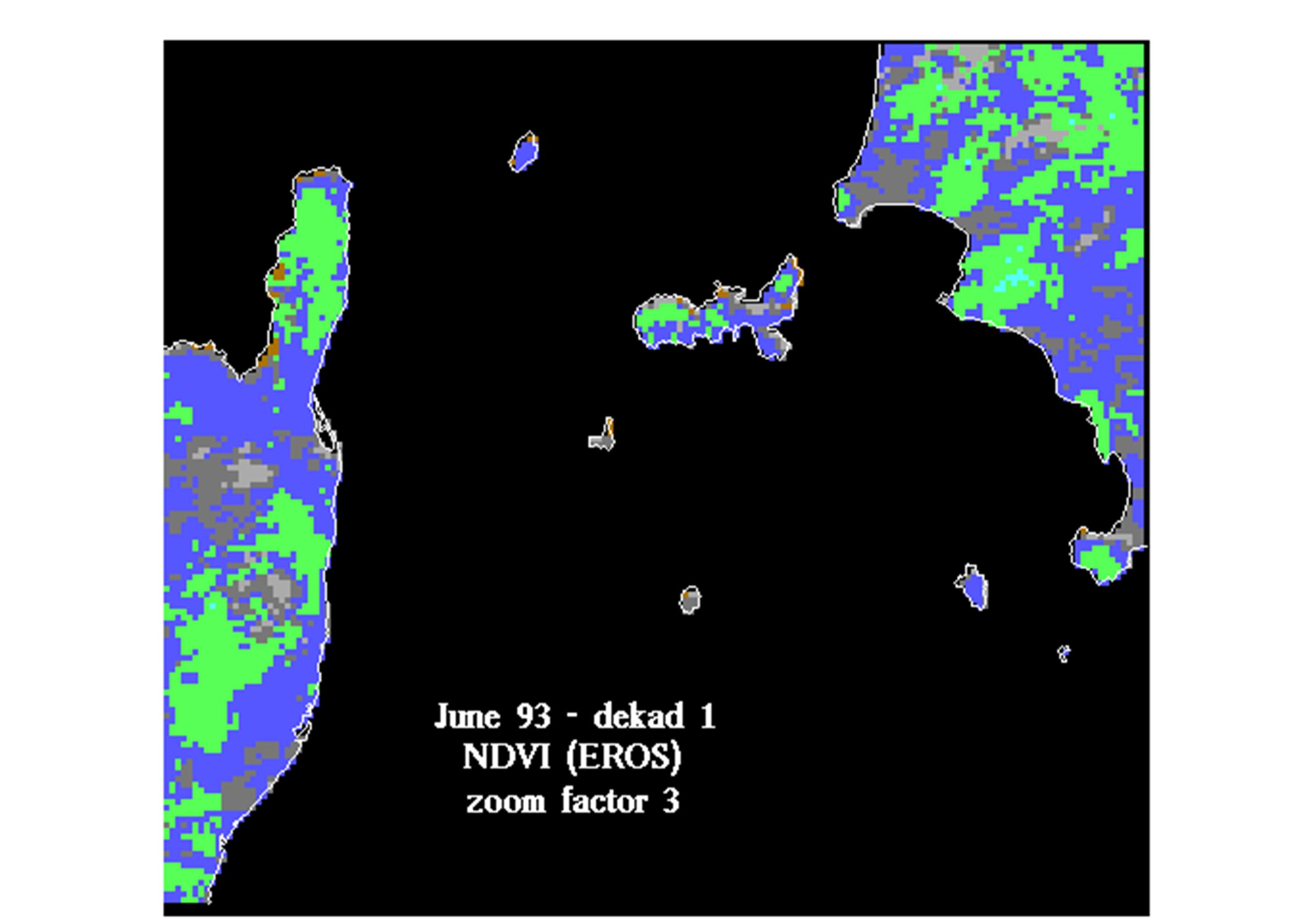
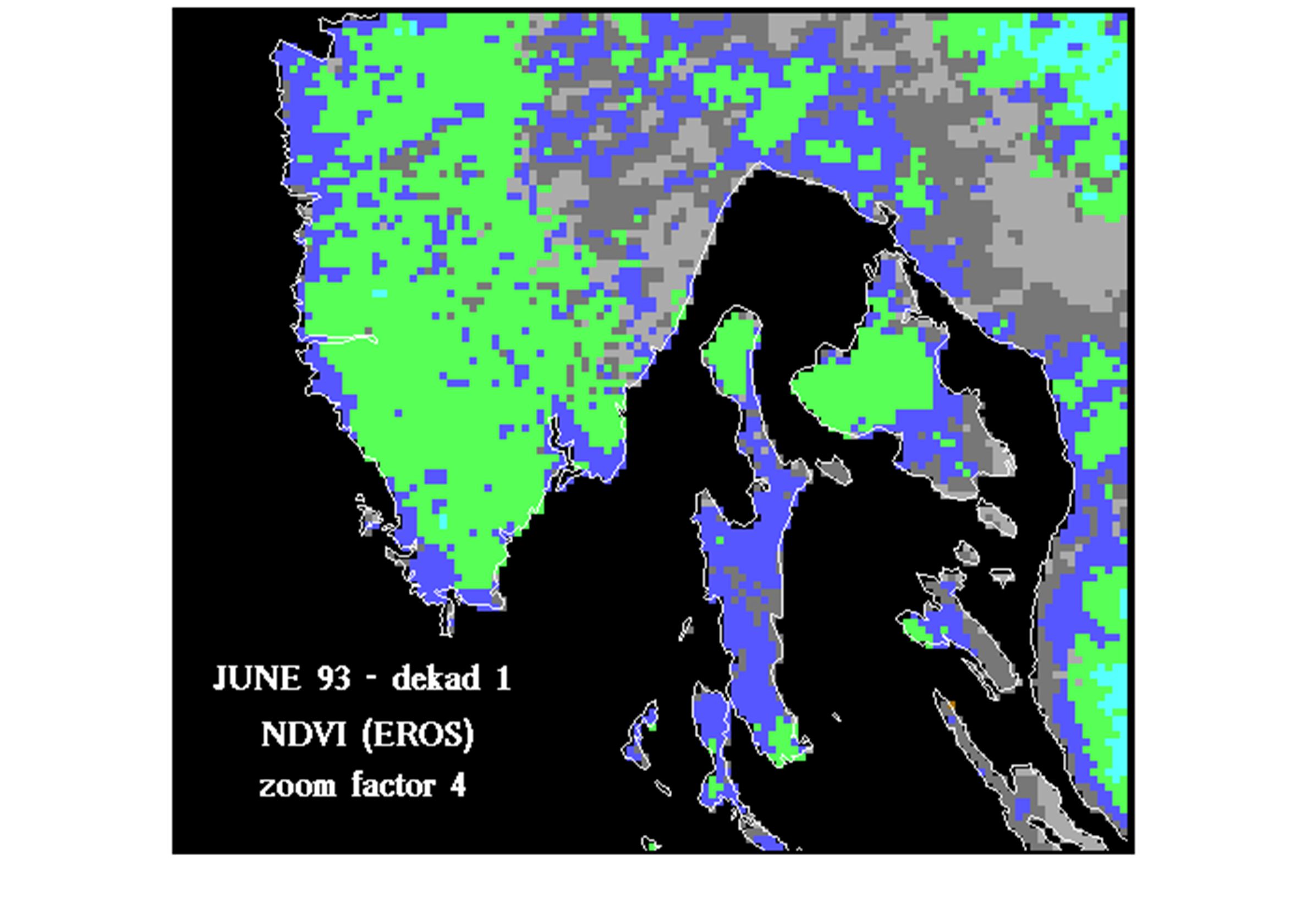
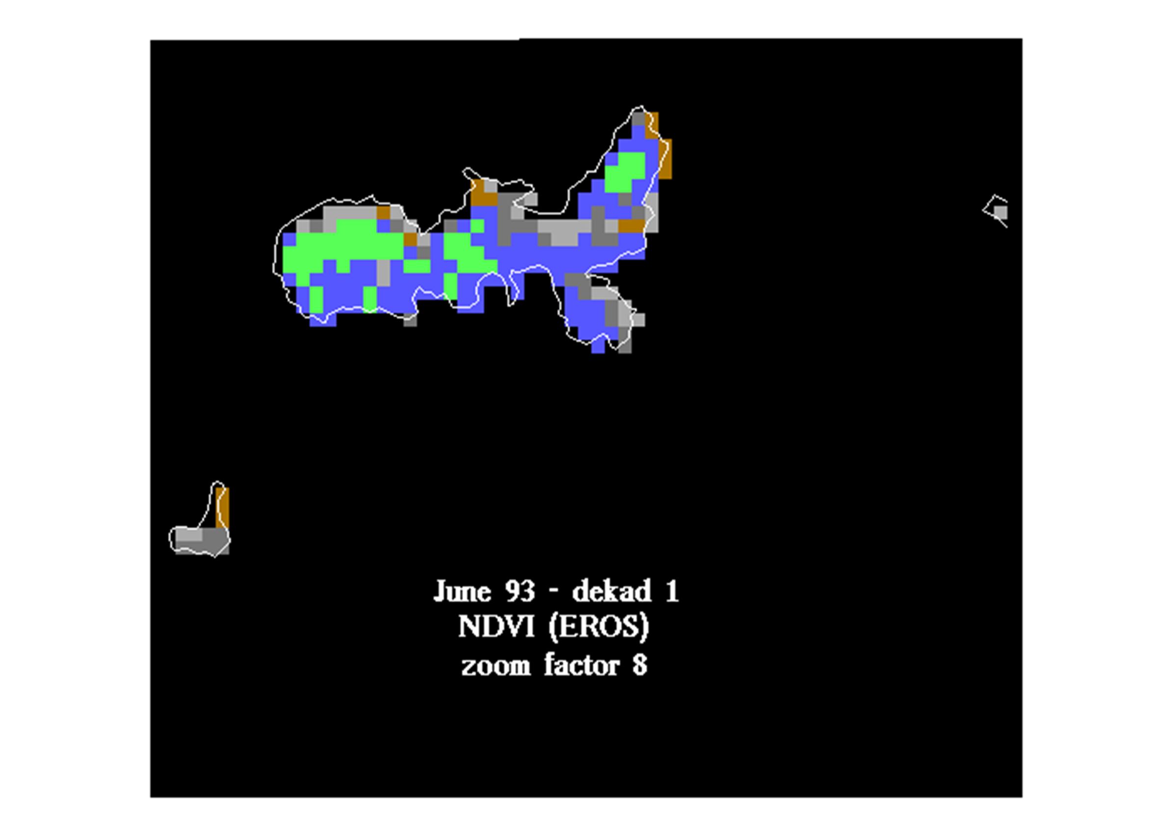
Le immagini EROS sembrano buone? Chissà…
E’ stata applicata una maschera all’acqua, non è dato sapere quanto ben registrate fossero le immagini daily usate per costruire le MVC. Anche quelle MARS diventerebbero accettabili (almeno in apparenza) se si mascherasse l’acqua. Ma il “blurring” rimane.
 se. si mascherasse l’acqua. Ma il blurring rimane.")
48
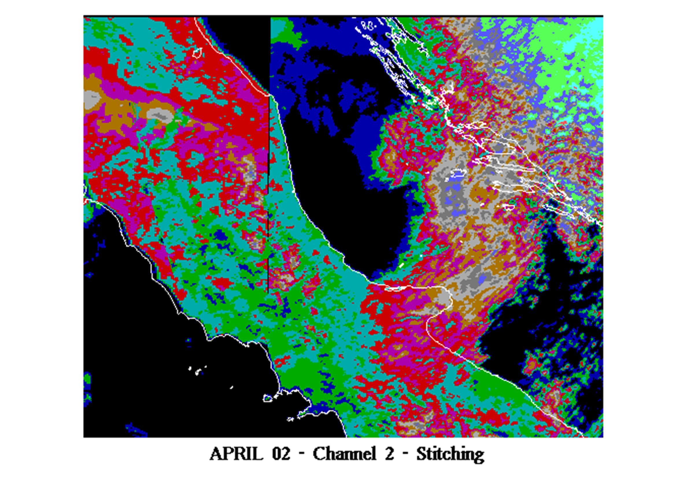
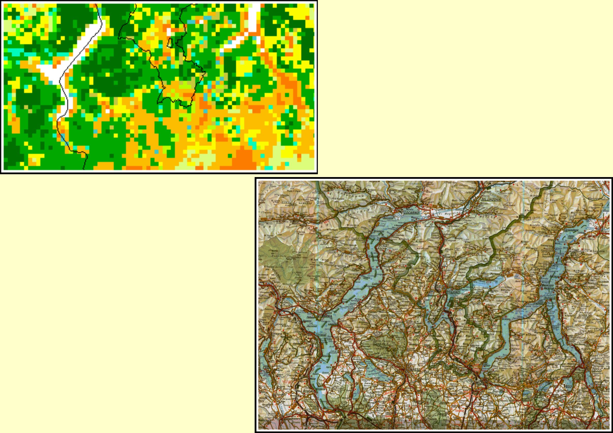
Immagini SMART 1991: la registrazione sembra buona...

49
…ma quelle relative al 1997, non mascherate, sono meno convincenti
Esempio di “blurring” causato dalla cattiva registrazione delle immagini giornaliere usate come input

51
But first, some basic terms and concepts...

52
Some open questions... But first of all...
Statistical or neural? Which type of Classifier to use? supervised or unsupervised? Which clustering method? But first of all... Is the satellitary information alone sufficient? Generally NO, it is necessary to have recourse to some auxiliary information to solve dubious cases. (insufficience of the description).
.")
53
Pixels can be grouped (or clustered) in classes:
Image pixels: geo-referenced statistic units, described by a suitable set of characters (spectral bands, images observed at different dates, synthetic images, ecc.). (the description is multidimensional) Pixels can be grouped (or clustered) in classes: according to their similarity with some pre-defined themes, represented by a set of suitably selected pixels supervised methods; or according to their similarity with one another un-supervised (constructive-exploratory) methods;
![]()
54
Principal Components Analysis (PCA)
Channel values used as variables are often higly correlated. A PCA is used to convert the initial variables to new latent variables, called Principal Components, that are uncorrelated. This operation: reduces the dimensionality of the description filters out noise (i.e., casual, unimportant, non- structural aspects). A PCA is often applied before clustering, to save computation time.
. A PCA is often applied before clustering, to save. computation time.")
55
Assumption two pixels are similar when they lie close to each other in the feature space (this depends on the way the distance is defined). Create groups (classes) as compact as possible in the feature space To cluster
![]()
56
Now, a short description
of the main approaches for clustering...

57
Supervised methods Problems are given a priori;
The target-themes (water, built-up, vegetation, etc.) are given a priori; A suitable training set must be defined. The theme to which any pixel included in the training set belongs must be explicitly stated. The classifier learns from the training set to recognize the themes’ features, and to assign all new pixels to the most appropriate theme. Problems Pixels are generally mix of different themes The construction of the training set is a hard and error-prone job.
 are given a priori; A suitable training set must be defined. The theme to which any pixel included in the training. set belongs must be explicitly stated. The classifier learns from the training set to recognize the themes’ features, and to assign all new pixels to the most appropriate theme. Problems. Pixels are generally mix of different themes. The construction of the training set is a hard and. error-prone job.")
58
Statistical supervised Classifiers
maximum likelihood minimum Mahalanobis distance Neural supervised Classifiers BackPropagation

59
Unsupervised methods (esploratory)
themes are not defined a priori; pixels are grouped according to the similarity of the patterns that describe them; the meaning of the groups thus obtained must be assessed ex-post (interpretation).
.")
60
Problems with unsupervised methods
The classification is optimal from the viewpoint of the algorithm, but... classes are built upon the most frequent patterns; therefore, the meaning of the groups is often not neat; rare patterns, albeit well characterized, are unable to get a specific class allocated for them.

61
Statistical unsupervised Classifiers
numerous methods (mostly variants of the k-means) minimum Internal Inertia (or Variance within groups) Neural Unsupervised Classifiers Kohonen’s Self Organizing Maps (SOM) gli esempi presentati alla rete consistono solo di un insieme di pattern (vettori di attributi), classificati per similarità. Ad ogni nodo (i, j) della mappa è associato un vettore di riferimento m i,j (codebook)
 minimum Internal Inertia (or Variance within groups) Neural Unsupervised Classifiers. Kohonen’s Self Organizing Maps (SOM) gli esempi presentati alla rete. consistono solo di un insieme di. pattern (vettori di attributi), classificati per similarità. Ad ogni nodo (i, j) della mappa. è associato un vettore di. riferimento m i,j (codebook)")
62
Kohonen’s Map The pixel with pattern x is assigned to class (1,1)
![]()
63
Reti SOM - procedura di istruzione
Ciascun pattern x viene confrontato con tutti i vettori mij ed assegnato al nodo associato al vettore mij più somigliante. Il nodo vincitore e quelli vicini vengono modificati in modo da accentuare la loro somiglianza con il pattern x. Una SOM sviluppa in modo autonomo durante la fase di apprendimento un’organizzazione interna: pattern di ingresso simili attivano lo stesso nodo della mappa. Le applicazioni sono di carattere esplorativo

64
Primi esperimenti di classificazione...
Classificazione non supervisionata Classificazione semi-supervisionata Reti Neurali Classificazione supervisionata (Mahalanobis)
")
68
The windows chosen to train the classifier….

69
Details from the classified image issued by a classifier
trained on selected ares. Built-up areas are split into two density zones.

70
Calcolo sistematico di distribuzioni statistiche spaziali

71
PELCOM ha 11 temi, da suddividere in sub- temi quando possibile
Statistiche sulla distribuzione dei temi calcolate da CORINE e dal DTM (quote). Sistematicamente, per ogni tema ed ogni area. Obiettivo: aiutare l’interpretazione delle classi, formulare opportune regole di post-classificaziome CORINE ha 43 temi PELCOM ha 11 temi, da suddividere in sub- temi quando possibile
. Sistematicamente, per ogni tema ed ogni area. Obiettivo: aiutare l’interpretazione delle classi, formulare. opportune regole di post-classificaziome. CORINE ha 43 temi. PELCOM ha 11 temi, da suddividere in sub- temi quando possibile.")
72
North Italy (ITN) - Distribuzione di temi sulla quota
 - Distribuzione di temi sulla quota")
73
North Italy - Distribuzione di temi sulla quota

74
Italia Centrale - Distribuzione di temi sulla quota

75
Vigneti ITC Distribuzione spaziale dei temi Vigneti, Oliveti Oliveti

76
ITS Distribuzione spaziale dei temi Aree irrigate

77
Puglia (ITP) Distribuzione dei temi sull’elevazione Aree irrigate
 Distribuzione dei temi sull’elevazione Aree irrigate")
78
Altre statistiche per area
e tema: serie storica dell’ Indice di Vegetazione (NDVI) Non molto confortante ..
 Non molto confortante ..")
79
Determinazione di regole di decisione (post-classificazione)
")
80
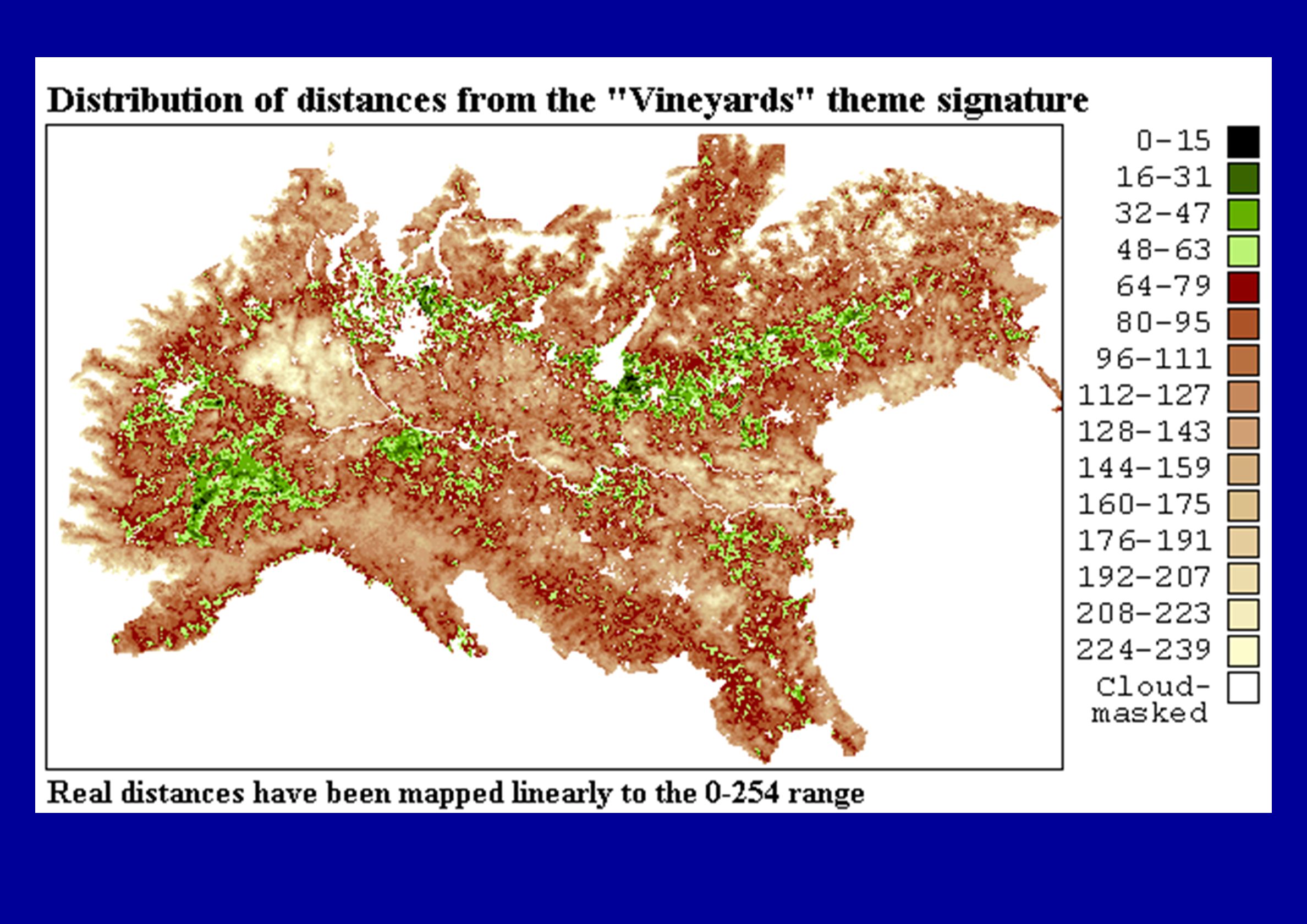
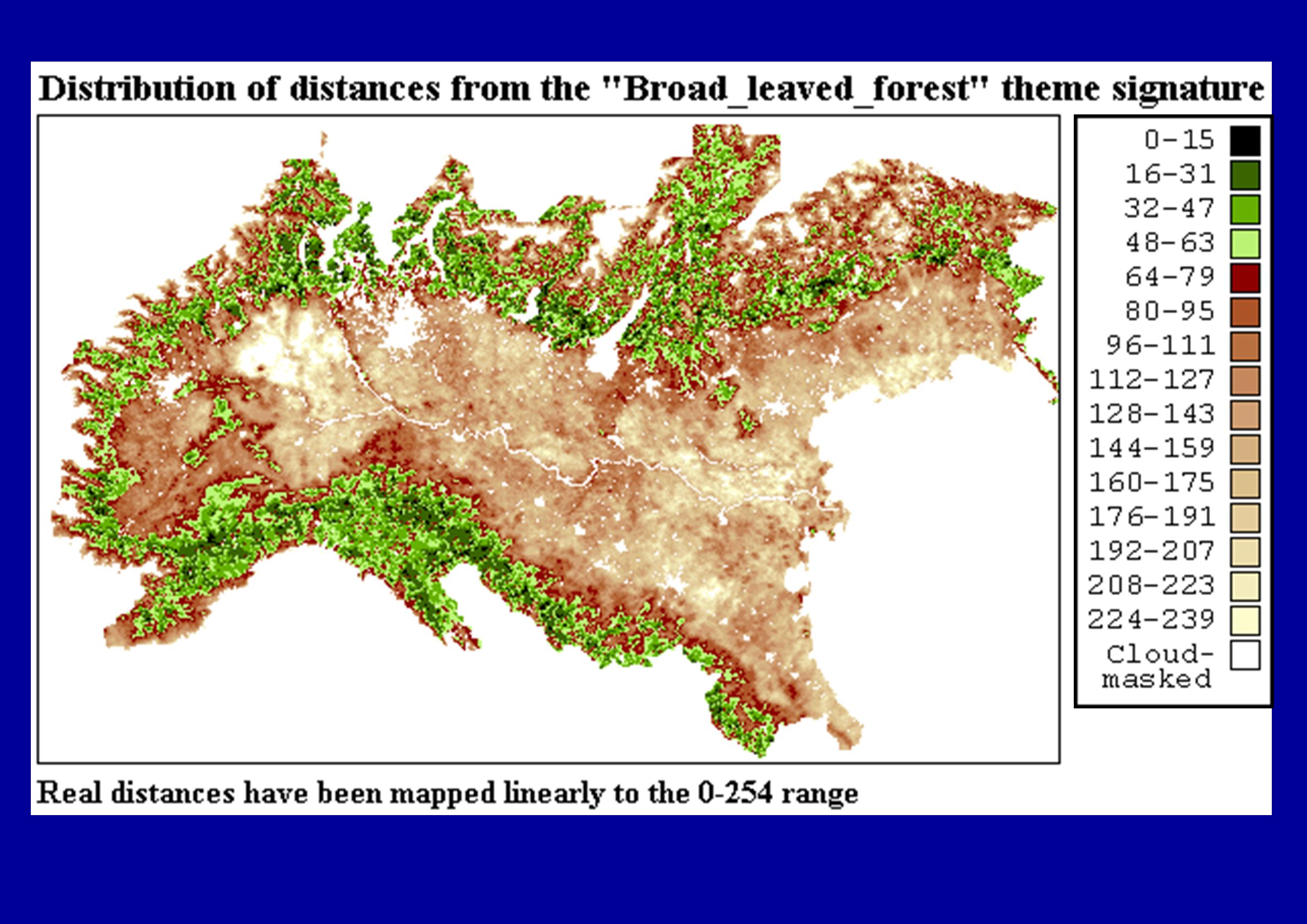
Altre statistiche per area e tema calcolate durante le
classificazioni: mappe raster della distanza dei pixel dai temi (rappresentati dalla firma spettrale calcolata a partire dai pixel di addestramento)
")
83
Clustering Methodology
Selection of training pixels Knowledge-based Classification Validation

84
Strongly methodological, the work concerned mainly:
the optimal territorial stratification; the choice of the images to be used; extended experimental comparison of the available clusering methods Eventually, a supervised method was chosen that included: an original way of choosing the training pixels; the direct utilization of available ancillary information within the clustering procedure itself.

85
The Classification Variables: 20 images NDVI during year 1997, produced by DLR, Berlin; Training pixels: for each theme, a set of pixels were chosen in each region, that were sufficiently pure in CORINE. Ancillary information: CORINE, Digital Terrain Model at 1 km., Digital Chart of Forests, Bartholomew Maps, FIRS strata, administrative statistics, etc.

86
1. Choice of training pixel
(the method can be easily extended to Neural Network Classifiers)
![]()
87
Distribution of training pixels
used for Italy in PELCOM. For each area of interest, a certain number of “pure” pixels (at least 87% belonging to the same theme in CORINE) have been selected, and used to train the classifier. All other pixels are then assigned to the most similar group.
![]()
88
ITN - Projection of candidate training pixels onto the first factor
plane. For most themes the level of confusion is high.
![]()
89
Confusion matrix for initial training pixels
Columns: pixels theme in CORINE. Rows: theme to which pixels are assigned by the classifier, after computing the themes’ signatures.
![]()
90
Selection of the most reliable training pixels
(repeated for each region) Initial selection of all candidates (14/16 pure CORINE) Computation of the signatures for all relevant themes Assignment of each training pixel to the closest signature according to the Mahalanobis distance, thus keeping into account the dispersion of each theme in the reference space Too many ill-classified pixels? END no yes Exclusion of ill-assigned pixels
![]()
91
ITN - Training pixels retained after several iterations
ITN - Training pixels retained after several iterations. Confusion is much reduced.
![]()
92
Confusion matrix for the finally selected training pixels
Columns: pixels theme in CORINE. Rows: theme to which pixels are assigned by the classifier, after computing the themes signatures.
![]()
93
2. Clustering Method that makes use of
the available ancillary information (Knowledge-based Classification) (Can it be applied to a Kohonen’s SOM NN?)
 (Can it be applied to a Kohonen’s SOM NN )")
94
The ancillary info used
while clustering: For each AoI, the distribution of each theme over altitude

95
Problems with clustering
At the 1.1 km scale pixels are mix of themes, their spectral signatures are averages; The profiles of some themes are very similar; A classification purely based upon radiometric data can sometimes lead to unreliable or absurd results: Example: arable land pixels detected at high elevation, owing to their similarity with bare soil.

96
How should pixel be assigned?
In two steps: 1. Purely according to the similarity of their profiles (with much confusion)… 2. … then applying some suitable decision rules to correct the results. Or Knowledge-based Classification …making use of some relevant ancillary information during the very clustering process.
![]()
97
The Knowledge-based Classification Algorithm
1. Selection of a set of reliable training pixels 2. For each active theme: computation of the average signature computation of the specific variance-covariance matrix and of its inverse (needed to compute Mahalanobis distances) 3. The elevation is divided in user-defined intervals and the table Target that cross-tabulates themes vs. elevation ranges is computed from CORINE. 4. Target is corrected by taking into account also contributions to active themes coming from pixels that belong in CORINE to non-active themes.
 3. The elevation is divided in user-defined intervals and the table Target that cross-tabulates themes vs. elevation ranges is computed from CORINE. 4. Target is corrected by taking into account also contributions to active themes coming from pixels that belong in CORINE to non-active themes.")
98
5. Pixels are assigned to active themes according to the Mahalanobis distance. This is based purely on pixels’ signature. For each pixel, the Mahalanobis distances from all active themes are saved to a temporary file. The table Current of themes’ frequency vs. elevation is computed. 6. At this point we have two matrices: Target: themes versus elevation as in CORINE Current: themes versus elevation as computed from clustering
![]()
99
Common structure of matrices Target and Current:
The classification is changed iteratively so as to have the computed table Current better match the knowledge base (CORINE) represented by Target; at the same time, also Target is slightly modified so as to keep somehow into account info in input data. Common structure of matrices Target and Current: n user-defined elevation ranges; p active themes; Cij is the frequency of theme j at elevation range i in the Current table; on each iteration, assignment to cell (i,j) - is encouraged if Cij < Tij - is dis-couraged if Cij > Tij
 represented by Target; at the same time, also Target is slightly modified so as to keep somehow into account info in input data. Common structure of matrices Target and Current: n user-defined elevation ranges; p active themes; Cij is the frequency of theme. j at elevation range i in the Current table; on each iteration, assignment to cell (i,j) - is encouraged if Cij < Tij. - is dis-couraged if Cij > Tij.")
100
7. A table of correction factors CFij (also sized n x p) is defined
7. A table of correction factors CFij (also sized n x p) is defined. Initially they are all equal to 1. Each correction factor refers to one cell. CFij is used to correct the Mahalanobis distance from theme j of pixels at elevation range i. 8. A cicle of iterations is started, aimed at orienting the assignments (no hard constraints), so as to encourage Current to adhere to Target. At the same time also Target is corrected (though less), moving it towards Current.
 is defined. Initially they are all equal to 1. Each correction factor refers to one cell. CFij is used to correct the Mahalanobis distance from theme j of pixels at elevation range i. 8. A cicle of iterations is started, aimed at orienting the assignments (no hard constraints), so as to encourage Current to adhere to Target. At the same time also Target is corrected (though less), moving it towards Current.")
101
One iteration (cycle 9-10 is repeated)
9. For each pixel: re-read its Mahalanobis distances from file, and correct each with the correction factor CFij appropriate to the theme and to the pixel’s elevation; assign the pixel to the theme for which the so-corrected Mahalanobis distance is minimum. 10. Update the Current distribution Update the correction factors: Update Target

102
V A L I D A T I O N ( 1 ) All AOIs - 12/16 pure pixels (not used for training) Columns: theme of pixel in CORINE. Rows: theme to which pixel is assigned by the classifier.
![]()
103
V A L I D A T I O N ( 2 ) All AOIs - 12/16 pure pixels (not used for training) Columns: theme of pixel in CORINE. Rows: theme to which pixel is assigned by the classifier. Forests are aggregated, as well as grassland/pastures.
![]()
104
Remarks frequent themes, like arable or deciduous, are well classified; less frequent themes, like permanent crops, coniferous or grassland, are better classified in AOIs for which enough training pixels can be found; when the classification was attempted with only few training pixels (pastures or permanent crops in some areas), results were unreliable;
, results were unreliable;")
105
An excerpt of Validation tables- summary per theme
Non-irrigated arable land

106
Irrigated arable land + Rice

107
ITS - Spatial distribution of irrigated land

108
A3 - Spatial distribution of irrigated land

109
Permanent Crops

110
Conclusions When the target themes are pre-defined, a supervised
classifier is convenient. Statistical and neural methods lead to results of comparable accuracy. The methods used with statistic classifiers in order to select optimally the training pixels, as well as the knowledge-based classification, should be extended to neural classifiers.

111
The Natural Capital Index (NCI)
enables to monitor and describe the current and future State of the Environment

112
} Principle Natural Capital Index: NCI = quantity x quality
100% 0% quality quantity NCI = quantity x quality Quantity: % area Quality : % baseline state } “gap-analysis” self-regenerating current / natural baseline man-made current / cultural baseline

113
Self-regenerating areas are defined as:
“all not human-dominated land, irrespective of wether it is pristine or degraded” virgin land, nature reserves; all forests except wood plantations with exotic species; areas with shifting cultivation; all fresh water areas; and extensive grasslands (marginal land used for grazing by nomadic livestock).
.")
114
Man-made Areas are defined as:
“all human-dominated land” arable land; permanent cropland; wood plantations with exotic species; pasture for permanent livestock; urban areas; infrastructure; and industrial areas. Most domesticated land is in fact agricultural land.

115
Self regenerating land in PELCOM database

116
Pressures to biodiversity with respective standardizing values

117
Pressure index in remaining self-regenerating land (1990)
Based on: Ozone Isolation Temperature GDP Acidification Eutrofication

118
NCI statistics (1990) on Eu-country level
 on Eu-country level")
119
Pressure index in remaining self-regenerating land (baseline 2010)
Based on: Ozone Isolation Temperature GDP Acidification Eutrofication

120
NCI statistics (2010) on Eu-country level
 on Eu-country level")
121
Conclusions II NOAA derived land cover data are an important and
accurate source of input data for current NCI calculation The consistent classification for the entire pan-European area is the most important added value of PELCOM

Presentazioni simili


 Brussels, 26 settembre 2013.>")
 064825120 - fax.>")


>")


>")
>")
