Normalmente i velocimetri Doppler forniscono il segnale audio corrispondente al Doppler shift ed un segnale video già elaborato (sonogramma), convenzionalmente.

Presentazione sul tema: "Normalmente i velocimetri Doppler forniscono il segnale audio corrispondente al Doppler shift ed un segnale video già elaborato (sonogramma), convenzionalmente."— Transcript della presentazione:

1 Normalmente i velocimetri Doppler forniscono il segnale audio corrispondente al Doppler shift ed un segnale video già elaborato (sonogramma), convenzionalmente riportato nella parte sup e inf dello schermo a seconda che corrisponda al canale in avvicinamento o in allontanamento. L’elaborazione avviene tramite una serie di processi che sono descritti nel seguito.

2 Signal acquisition The first step is sampling  the signal (possibly any period T ) is segmented in time intervals Dt: Dt = T / N Buona risoluzione temp: Dt piccolo N grande

3 Il numero N di campioni per periodo è la frequenza di acquisizione, o sampling frequency: fs = N/T. Dovendo riconoscere le frequenze presenti nel campione occorre trasformare secondo Fourier: in pratica si usa la FFT, che viene applicata su un numero di punti N = 2 k. ( es: 512 o 1024). La risoluzione in frequenza è data da Df = fs/N Df Buona risoluzione in frequenza: Df piccola  N grande, k grande

4 Che limitazioni ci sono su N e su k? Innanzitutto N deve essere una potenza di 2 (il che non è un problema…). Cominciamo dal caso di un segnale stazionario: campionerò un certo blocco di N dati su cui applicherò la FFT. Se lavoro su di un unico blocco, avrò una certa quantità di rumore sovrapposto al segnale. L’unico modo di ridurre il rumore consiste nel campionare molti blocchi e mediare il risultato sui blocchi: FFT

5 Se prendo blocchi troppo lunghi (N grande) non potrò mediare molti blocchi, perché ho un limite sul buffer. Se scelgo k troppo grandi, avrò una buona risoluzione in frequenza ma impiego molto tempo per la FFT di singolo blocco: non ho una procedura in tempo reale. Conviene dimensionare k in modo che il tempo di FFT sia inferiore al tempo di campionamento, e usare i blocchi di dati in condizione di overlapping: FFT

6 Nel caso in cui il segnale sia periodico, es flusso unsteady, i vincoli sono maggiori, perché non possiamo mediare su blocchi in overlapping, ma soltanto su intervalli di tempo corrispondenti: Poniamo di voler studiare il periodo suddividendolo in n intervalli: allora mi servono N= 2 k * n punti. Se f è la frequenza del segnale: fs = N f  a seconda di f conviene modificare fs. Ad es: A parità di N=10240 f(Hz) fs(kHz) tempo acq (s) 0.1110.24 1101.024

7 Un altro punto importante: l’ aliasing. La scelta della frequenza di campionamento non è casuale, ma dipende dal segnale campionato… FFT trasforma gli N punti campionati in N/2 intervalli equidistanti di frequenza. Questo significa che la massima frequenza che può riconoscere sarà data da: fmax=N*Df /2= N*fs/2*N=fs/2 La frequenza di campionamento deve essere almeno doppia della massima frequenza che voglio riconoscere nel segnale! (criterio di Niquist)

8 Se non rispetto questa prescrizione si crea una frequenza fittizia fs-fmax che ‘sporca’ il segnale e lo deforma. Se rispetto la prescrizione la frequenza di aliasing si viene a formare sulla destra della fmax, e può essere facilmente filtrata Df

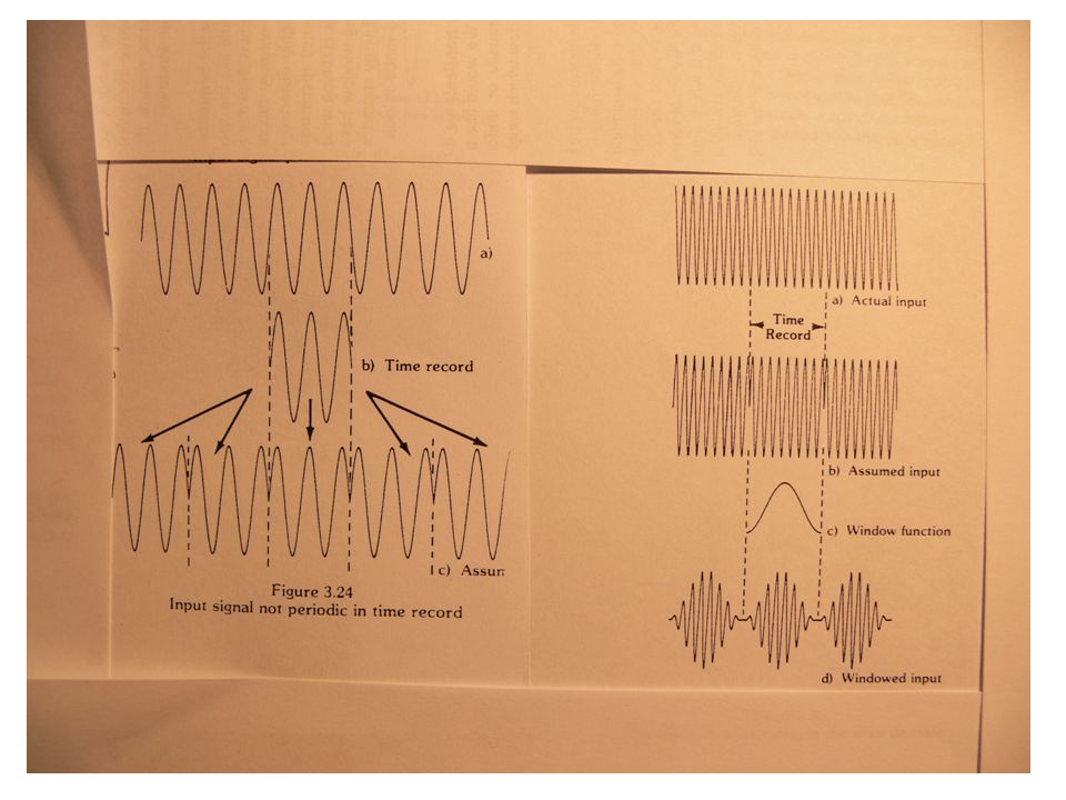
9 Un’ ennesima difficoltà: il leakage Supponiamo di avere un segnale periodico e di campionarlo senza rispettare la sua periodicità: Questo introduce delle frequenze fittizie nel segnale! La stessa cosa succede per un segnale qualsiasi. Poiché il problema si presenta ‘ai bordi’ del blocco di campionamento, esso viene ‘risolto’ introducendo una finestra di campionamento, o ‘windowing’, che riduce il peso dei campioni alla periferia rispetto a quelli centrali:

10

11 Ancora un problema sulla frequenza massima: come distinguerla dal rumore? Quando le ampiezze diventano molto piccole, i segnali diventano estremamente evanescenti. Occorrono tecniche particola- ri per valutarle: algoritmi adattativi. Un esempio è quello proposto da D’Alessio e colleghi (1985): Dfn Th r0r0

12 In the power spectrum, the Doppler signal is revealed only when in m consecutive spectral lines, at least r 0 of them exceed a fixed threshold value T h, which changes depending on the noise level. Therefore, the maximum Doppler frequency is at the first line exceeding the boundary. The spectral noise density N 0 is obtained by averaging, for any spectrum, the n lines with higher frequency. The probability P sp that, when only the noise is present, a signal doesn’t be shown, is determined by the parameters m and r 0, while the probability P th,n that a spectral line exceeds the threshold T h, is function of P sp and m and given by: Moreover, the correct individualisation of a signal, in presence of noise, depends on the signal to noise ratio SNR.

13

14 3.5 The acquisition system A PC acquisition method is used in our laboratory. The signal, trough the tape output of the instrument is taken upstream the processing, acquired and digitalised with a LAB 1200 card National Instrument and a Pentium III PC. Both the acquisition and the following data analysis are administrated with a program written in LabView (Laboratory Virtual Instrument Engineering Workbench) environment, a graphic programming system of the National Instruments. LabView employs the so-called G language: it is a very intuitive method, which allows to develop a program, using some objects, called virtual instruments (VIs), which are connected among them, simulating real scientific devices.

15 Any LabView program or Virtual Instrument has a front panel and a block diagram. In this case, the front panel is the user graphical interface of the LabView 6. This interface collects all user inputs and shows program outputs. Buttons, keys and other indicators can be present. The block diagram contains the source code of the system graphical part.

16

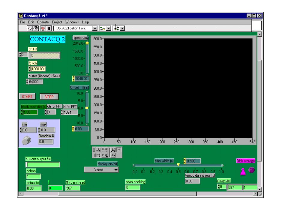
17 In the upper part, on the left side, there are the input variables: -first, the window of the acquired channels list, -then the sampling frequency (10 kHz) -and the buffer (64000). -The information about FFT, channel (0) and points number (1024) are shown under the START and STOP buttons. In the centre of the panel, a screen to visualize both the signal and the PDS is present: a key under it allows to select both alternately. Next to it, a bar represents the temporal amplitude of the sampling. Finally, in the lower part of the panel, on the right side, a switch can record the signal on the disk. It is worth noting that this program can be used only to acquire a steady flow, while in the case of pulsatile movement an other block diagram must be considered. In fact, some differences are present, because, in the unsteady conditions, a sinusoidal wave is superimposed to a constant frequency and a modulation effect is obtained. A trigger signal begins any period of the pulsating wave. In the following figure, the front panel of this other program is shown:

18 Its structure and many buttons are the same as in the steady case, but, here, it is also possible to change other parameters, as -the epoch length, i.e. the acquisition duration (starting from each trigger pulse), - the minimum delay between epochs, that is the minimum time period that must elapse between one trigger pulse and the next ‘active’ one (trigger pulses rise before that this time is disabled) and the read timeout: the read block is locked until the whole epoch is acquired or until this timeout is reached.

19 Il processing:

20 Cosa c’è dietro? Occorre acquisire anche lo schema Sia nel caso steady sia nel caso unsteady

21 Steady case

22 Unsteady case

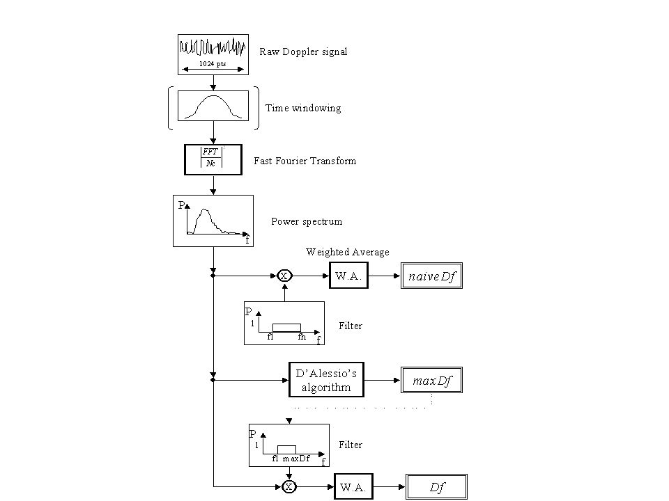
23 First, the signal is processed using a time windowing, which can be chosen among a rectangular or Hamming’s or Hanning’s one, to avoid that the non periodicity of the signal may cause artefacts. The Doppler spectrum is, at the beginning, evaluated with a raw FFT, for periods of 0.1 s: this time is considered rather short to assure the signal stationariness, as requested from the FFT algorithm. Starting from any spectrum, calculated with a particular time windowing, different parameters are extracted and then averaged on a time period of at least 1 s. The first of them is the average Doppler shift, which is the mean frequency of the power spectrum obtained as the weighed average of the all spectral lines in the whole range defined during the acquisition procedure (i.e. between f l and f h, which are the cutting off frequencies of the band pass filters of the Doppler system). Since the used algorithm is very raw, this average Doppler shift is called ‘naïve’ (Guiot et al, 1997). Successively, the maximum and the correct mean frequency are obtained making use of the D’Alessio algorithm. Finally, it is also possible to extract the signal to noise ratio, SNR.

24 In the left side of the panel, the same parameters of the acquisition program are present, even if, in this case, it is possible to select the channel to analyse. In the post processing part, you can choose the time interval, when to process the signal and in the four windows below, the numerical values and the standard deviation of SNR, mean maximum frequency, mean naïve frequency and mean correct frequency are shown. Then, through the two green buttons in the ‘show spectrum’ section, it is possible to visualise and record the spectrum. In the right side of the panel, there is the screen, where the four parameters considered before are graphically represented. Below it, some keys can change the range, to conform it to the estimated values. Above it, data about processing, data and FFT dimension, the kind of time windowing, the number of noise samples are shown and other parameters requested from the D’Alessio algorithm can be read.

25 Also in this case, different programs are needed for steady and pulsatile flow. The front panel is practically the same, with the only difference that a button to record all spectra in any points of the period was added. It is also possible to save the values of the different parameters for any points of the periods, so, in this way, you can average values on the correspondent time interval from many periods. This is very useful to remove a lot of noise from the signal and recognize the forced waveform.