Riccardo Valentini Università della Tuscia

Presentazione sul tema: "Riccardo Valentini Università della Tuscia"— Transcript della presentazione:

1 Ecosystems and global services : an outlook on forest and mountain region
Riccardo Valentini Università della Tuscia Dipartimento di Scienze dell’Ambiente Forestale e delle sue Risorse

2 Welcome in the Anthropocene !
CH4 N2O

3 2007 un anno per il Clima 4° Rapporto Intergovernativo sui Cambiamenti Climatici Premio Nobel per la Pace Un film sul clima Artico si scioglie Bush torna su i suoi passi ? Il delfino Baiji è estinto

4

5 What was unique? Ecosystem services
Provisioning Goods produced or provided by ecosystems Regulating Benefits obtained from regulation of ecosystem processes Cultural Non-material benefits from ecosystems The assessment focuses on the linkages between ecosystems and human well-being and, in particular, on “ecosystem services.” An ecosystem is a dynamic complex of plant, animal, and microorganism communities and the nonliving environment interacting as a functional unit. The MA deals with the full range of ecosystems—from those relatively undisturbed, such as natural forests, to landscapes with mixed patterns of human use, to ecosystems intensively managed and modified by humans, such as agricultural land and urban areas. Ecosystem services are the benefits people obtain from ecosystems. These include provisioning services such as food, water, timber, and fiber; regulating services that affect climate, floods, disease, wastes, and water quality; cultural services that provide recreational, aesthetic, and spiritual benefits; and supporting services such as soil formation, photosynthesis, and nutrient cycling. The human species, while buffered against environmental changes by culture and technology, is fundamentally dependent on the flow of ecosystem services. Original version of this slide was prepared by Karen Bennett, WRI. Photo credits (left to right, top to bottom): Purdue University, WomenAid.org, LSUP, NASA, unknown, CEH Wallingford, unknown, W. Reid, Staffan Widstrand

6 See related Blue Marble imagery:
Figure not in MA. NASA Goddard Space Flight Center Image by Reto Stöckli (land surface, shallow water, clouds). Enhancements by Robert Simmon (ocean color, compositing, 3D globes, animation). Data and technical support: MODIS Land Group; MODIS Science Data Support Team; MODIS Atmosphere Group; MODIS Ocean Group Additional data: USGS EROS Data Center (topography); USGS Terrestrial Remote Sensing Flagstaff Field Center (Antarctica); Defense Meteorological Satellite Program (city lights). This spectacular “blue marble” image is the most detailed true-color image of the entire Earth to date. Using a collection of satellite-based observations, scientists and visualizers stitched together months of observations of the land surface, oceans, sea ice, and clouds into a seamless, true-color mosaic of every square kilometer (.386 square mile) of our planet. These images are freely available to educators, scientists, museums, and the public. This record includes preview images and links to full resolution versions up to 21,600 pixels across. Much of the information contained in this image came from a single remote-sensing device-NASA’s Moderate Resolution Imaging Spectroradiometer, or MODIS. Flying over 700 km above the Earth onboard the Terra satellite, MODIS provides an integrated tool for observing a variety of terrestrial, oceanic, and atmospheric features of the Earth. The land and coastal ocean portions of these images are based on surface observations collected from June through September 2001 and combined, or composited, every eight days to compensate for clouds that might block the sensor’s view of the surface on any single day. Two different types of ocean data were used in these images: shallow water true color data, and global ocean color (or chlorophyll) data. Topographic shading is based on the GTOPO 30 elevation dataset compiled by the U.S. Geological Survey’s EROS Data Center. MODIS observations of polar sea ice were combined with observations of Antarctica made by the National Oceanic and Atmospheric Administration’s AVHRR sensor—the Advanced Very High Resolution Radiometer. The cloud image is a composite of two days of imagery collected in visible light wavelengths and a third day of thermal infra-red imagery over the poles. Global city lights, derived from 9 months of observations from the Defense Meteorological Satellite Program, are superimposed on a darkened land surface map. See related Blue Marble imagery: Source: NASA

7

8 Global C Budget Fast process (1 – 102 days)
Atmospheric accumulation rate 3.2 GtC per year 1990s Atmosphere Surface biosphere 6.3 F Fuel, Cement 2.2 Land-Use Change 2.9 Land Uptake 2.4 Ocean Uptake Fast process (1 – 102 days) Slow process (103 – 104 days) Gruber et al 2003 , SCOPE project

9

10 Valentini, Dolman, Matteucci et al. Nature 2000

11 VULNERABILITY OF BIOSPHERE (feed-backs with carbon cycle)
Coupled carbon-climate models BIOSPHERE Source or sink ?

12 Vulnerability of Carbon Pools
Carbon in frozen soils: 400 PgC Carbon in wetlands: 450 PgC Carbon in tropical vegetation: 340 Pg Risk over the coming century of up to 200 ppm of atmospheric CO2 Not included in most climate simulations. Gruber et al. 2004

13 ……BIODIVERSITA’ IN CIFRE……
1,7 MILIONI DI SPECIE CONOSCIUTE 15 MILIONI SPECIE STIMATE SULLA TERRA 90% DELLE SPECIE SCONOSCIUTE

14 Change in Species Diversity
Number per Thousand Species Number of Species Homogenization (e.g. growth in marine species introductions) North America Europe 100 to 1000-fold increase MA Synthesis Figure SDM 4 (Extinctions) and Figure 1.7 Homogenization Figure 4. Species Extinction Rates (Adapted from C4 Fig 4.22) “Distant past” refers to average extinction rates as estimated from the fossil record. “Recent past” refers to extinction rates calculated from known extinctions of species (lower estimate) or known extinctions plus “possibly extinct” species (upper bound). A species is considered to be “possibly extinct” if it is believed by experts to be extinct but extensive surveys have not yet been undertaken to confirm its disappearance. “Future” extinctions are model derived estimates using a variety of techniques, including species-area models, rates at which species are shifting to increasingly more threatened categories, extinction probabilities associated with the IUCN categories of threat, impacts of projected habitat loss on species currently threatened with habitat loss, and correlation of species loss with energy consumption. The time frame and species groups involved differ among the “future” estimates, but in general refer to either future loss of species based on the level of threat that exists today or current and future loss of species as a result of habitat changes taking place over the period of roughly 1970 to Estimates based on the fossil record are low certainty; lower-bound estimates for known extinctions are high certainty and upper-bound estimates are medium certainty; lower-bound estimates for modeled extinctions are low certainty and upper-bound estimates are speculative. The rate of known extinctions of species in the past century is roughly 50–500 times greater than the extinction rate calculated from the fossil record of 0.1–1 extinctions per 1,000 species per 1,000 years. The rate is up to 1,000 times higher than the background extinction rates if possibly extinct species are included. Figure 1.7. Growth in Number of Marine Species Introductions (C11). Number of new records of established non-native invertebrate and algae species reported in marine waters of North America, shown by date of first record, and number of new records of non-native marine plant species reported on the European coast, by date of first record. From text on MA Synthesis SDM p. 4: “Humans are fundamentally, and to a significant extent irreversibly, changing the diversity of life on Earth, and most of these changes represent a loss of biodiversity. ■ Across a range of taxonomic groups, either the population size or range or both of the majority of species is currently declining. ■ The distribution of species on Earth is becoming more homogenous; in other words, the set of species in any one region of the world is becoming more similar to the set in other regions primarily as a result of introductions of species, both intentionally and inadvertently in association with increased travel and shipping. ■ The number of species on the planet is declining. Over the past few hundred years, humans have increased the species extinction rate by as much as 1,000 times over background rates typical over the planet’s history (medium certainty). (See Figure 4.) Some 10–30% of mammal, bird, and amphibian species are currently threatened with extinction (medium to high certainty). Freshwater ecosystems tend to have the highest proportion of species threatened with extinction. Plotting note for PowerPoint slide: To plot correctly, upper bound of fossil changed from 1 to .9 and upper bound of Future changed from to 9000 Extinctions (per thousand years) Source: Millennium Ecosystem Assessment

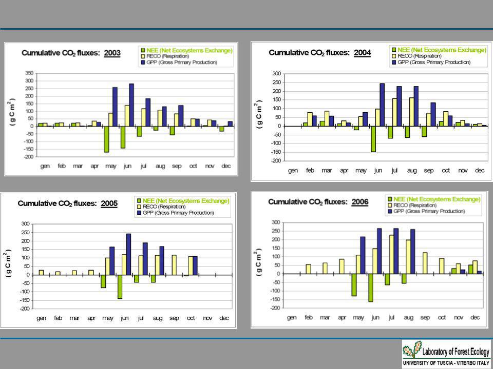
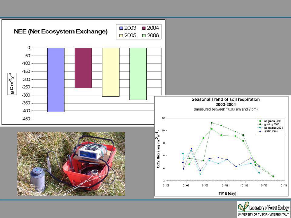
15 The experimental site is located in a farm (Malga Arpaco) at 1699 m a
The experimental site is located in a farm (Malga Arpaco) at 1699 m a.s.l. Mean annual temperature: 5 °C Total annual rainfall: 1200 mm Soil type: Typic Hapludalfs, fine loamy (FAO) Ecosystem type: alpine semi-natural grassland Ecosystem management: extensive management, pasture from Jun to Sep Period of EC measurements: Eddy Covariance type: Metek USA-1, Li-cor 7500 Tower height: 2 m

16

17

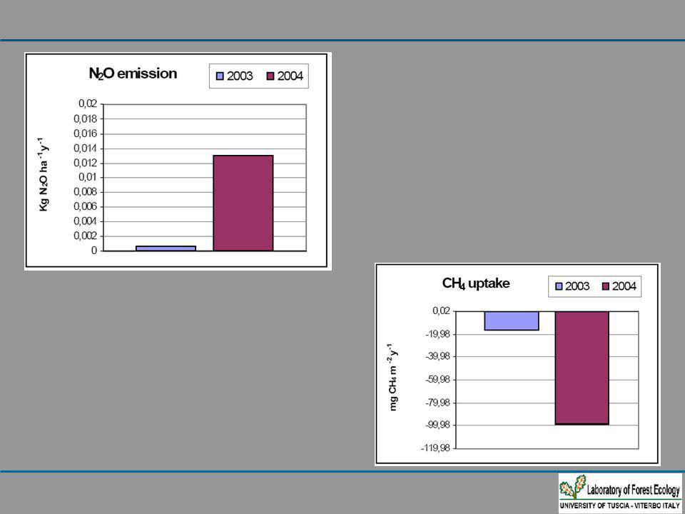
18 N2O emission and CH4 uptake was evaluated fortnightly, during
2003 and 2004 pasture season, using diffusion chambers. Gas samples conserved in vacuum vials were analysed through gaschromatography technique. For the N2O: ECD detector at 320°C; for the separation a capillary column Cromosob 1010 at 140°C was used, with a flux of helium at 30 kPa. For the CH4: FID detector at 180°C; for the separation a column 4m x ¼’’ OD Porapak q 80/100 MESH at 30° was used.

19

20

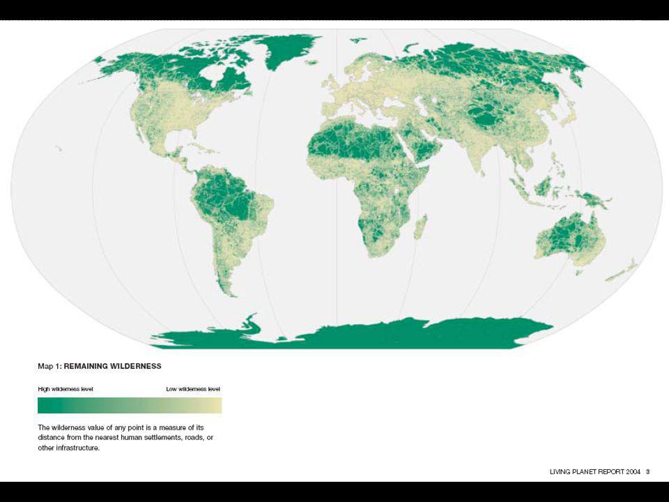
21 The human foot print Data Magnani et al., 2007

22 Luyssaert et al., submitted

23 53% wind throw 16% fire 16% biotic (insects) 3% snow 5% other abiotic
Extreme climate events or disturbances have a strong effect on biosphere-astmosphere exchanges Annual mean : 35 M m3 of forest wood damaged by natural disturbances in Europe. 53% wind throw 16% fire 16% biotic (insects) 3% snow 5% other abiotic Tatra Experiment CarboEurope

24 Malattie epidemiche causate da organismi introdotti
Vannini, Anselmi et al. 2007 Progetto CarboItaly QUALCHE ESEMPIO Malattie epidemiche causate da organismi introdotti Phythopthora cinnammomi, uno degli agenti causali del mal dell’inchiostro del castagno, è attualmente ristretta a quelle aree in cui la temperatura minima non scende al di sotto di 0°C (vedi grafico a destra). Un aumento delle temperature minime di 2-4°C, teoricamente verificabile nell’arco di anni, porterebbe questa specie ad espandere il suo areale alle zone castanicole dove sono oggi presenti specie di Phytophthora meno aggressive quali P. cambivora, P. cactorum e P. citricola La spiccata polifagia di P. cinnamomi, permetterebbe inoltre al patogeno di colonizzare nuovi ospiti precedentemente non raggiungibili per limiti climatici.

25 Malattie endemiche causate da organismi nativi
QUALCHE ESEMPIO Vannini, Anselmi et al. 2007 Progetto CarboItaly Malattie endemiche causate da organismi nativi Biscogniauxia mediterranea, è un fungo Ascomycota che vive comunemente come endofita indifferente all’interno dei tessuti corticali e legnosi di querce mediterranee. Durante eventi particolarmente siccitosi, quando il potenziale idrico fogliare minimo dell’ospite raggiunge valori inferiori a -2.0 MPa, la popolazione endofitica va gradatamente aumentando (vedi grafico) fino a quando, a valori inferiori a -3.0 MPa, il fungo passa dalla fase endofitica a quella patogenetica aggredendo rapidamente i tessuti dell’ospite e causando il cosiddetto “cancro carbonioso delle querce”. L’aumento delle temperature estive e la maggior frequenza di fenomeni estremi, tra cui la siccità, potrebbero “attivare” un alto numero di organismi comunemente “silenti” innescando pericolosi eventi di deperimento di cenosi forestali

26 Actual species distribution influencing distribution
Forest patterns Spatial modelling of forest patterns in dependence by location characteristics is a reliable way to analyze the possible trajectories and shifts of species habitat in the near future if environmental conditions will change. Actual species distribution Driving factors influencing distribution Statistical analysis Probability of occurrence Neighborhood criteria Future spatial distribution Scenarios of future driving factors

27 influencing distribution Actual species distribution
Driving factors influencing distribution Scenarios future driving factors Actual species distribution Statistical analysis Probability of occurrence Future Spatial Distribution Calibration Physiognomic categories % 00 - Woody plantation in agricultural areas 0.55 01 - Oaks and other evergreen broadleaf forests 9.07 02 - Deciduous oak-dominant forests 24.45 03 - Chestnut-dominant forests 8.85 04 - Beech-dominant forests 11.52 05 - Hygrophyte species-dominant forests 0.85 06 - Other broadleaf deciduous autochthon species-dominant forests 10.28 07 - Exotic broadleaf-dominant forests and plantations 1.85 08 - Mediterranean pine and cypress dominant forests 2.46 09 - Oro-Mediterranean and mountain pine dominant forests 2.75 10 - Abies alba and Picea rubens dominant forests 7.71 11 - Larch and cembrus pine dominant forests 3.06 12 - Exotic needleleaf dominant forests 0.10 13 - Mixed needleleaf and broadleaf forests with prevalent beech 2.19 14 - Mixed needleleaf and broadleaf forests with prevalent oro-mediterranean and mountain pine 2.24 15 - Mixed needleleaf and broadleaf forests with prevalent Abies alba and/or Picea rubens 1.93 16 - Mixed needleleaf and broadleaf forests with other species prevalent 6.77 17 - Tall Mediterranean Macchia 3.35 Forest Map of Italy (1:100000) raster 250 meters of resolution Error in rasterization -0.15% 26% of Italian territory is forest

28 influencing distribution Actual species distribution
Driving factors influencing distribution Actual species distribution Statistical analysis Probability of occurrence Future Spatial Distribution Scenarios future driving factors Calibration DEM srtm Driving factors Elevation values (m above sea level) Slope value (°) Aspect value (° clockwise from north) Mean annual precipitation (mm) Mean annual snow water equivalent (mm) Mean daily short wave net radiation (W/m2) Mean of the annual dew point temperature (°K) Mean of the minimum annual temperature (°K) Mean of the maximum annual temperature (°K) DMI F12 A2

29 Logistic regression Mean ROC 0.855
Driving factors influencing distribution Actual species distribution Statistical analysis Probability of occurrence Future Spatial Distribution Scenarios future driving factors Calibration Driving factors influencing distribution Actual species distribution Statistical analysis Probability of occurrence Future Spatial Distribution Scenarios future driving factors Calibration Logistic regression where Pi is the probability for the occurrence of the considered forest type on location i and the x's are the location factors (independent variable values) forcing the presence/absence of forest classes. Accuracy ROC 0.973 i.e.ROC curve test for class 8 Mean ROC 0.855

30 Example of Euclidean distance grid
Driving factors influencing distribution Actual species distribution Statistical analysis Probability of occurrence Future Spatial Distribution Scenarios future driving factors Neighbooring criteraia Calibration Driving factors influencing distribution Actual species distribution Statistical analysis Probability of occurrence Future Spatial Distribution Scenarios future driving factors Neighbooring criteraia Calibration Example of Euclidean distance grid Example of distance-based probability grid Piv

31 00 - Woody plantation in agricultural areas
Forest classes 00 - Woody plantation in agricultural areas 01 - Oaks and other evergreen broadleaf forests 09 - Oro-Mediterranean and mountain pine dominant forests 10 - Abies alba and Picea dominant forests 11 - Larch and cembrus pine dominant forests 12 - Exotic needleleaf dominant forests 13 - Mixed needleleaf and broadleaf forests with prevalent beech 14 - Mixed needleleaf and broadleaf forests with prevalent oro-mediterranean and mountain pine Altitude profiles of forest distribution Actual distribution Case a) Changed areas (red, 82%) considering only statistical analysis Case a) Case b) Changed areas (red, 77%) considering statistical analysis and neighborhood criteria Case b)

32 CONCLUSIONS Climate change will impact mountain ecosystems in different and possible unexpected ways (increase productivity, decrease biodiversity…) The human dimension is still important Conservation of old forests preserve ecosystem services

33 “You can observe a lot, just by watching.”
-Yogi Berra

34 Thank You