Disegno del modello di analisi dei dati sperimentali

Presentazione sul tema: "Disegno del modello di analisi dei dati sperimentali"— Transcript della presentazione:

1 Disegno del modello di analisi dei dati sperimentali
Lezione 3: Analisi della varianza (ANOVA)

2 disegno a blocchi randomizzzati
Tutti i trattamenti sono assegnati alle stesse unità sperimentali trattamenti sono assegnati ”random” C D A B blocchi (b = 3) trattamenti (a = 4)

3 trattamenti (Farmaci) blocchi (pazienti)
paziente A B C D media 1 2 3 trattamenti (Farmaci) blocchi (pazienti)

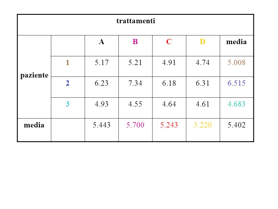
4 trattamenti paziente A B C D media 1 5.17 5.21 4.91 4.74 5.008 2 6.23 7.34 6.18 6.31 6.515 3 4.93 4.55 4.64 4.61 4.683 5.443 5.700 5.243 5.220 5.402

5 paziente 3 Farm. B

6 Valori Predetti di y

7 trattamenti paziente A B C D media 1 5.17 5.049 5.21 5.306 4.91 4.849 4.74 4.826 5.008 2 6.23 6.557 7.34 6.813 6.18 6.357 6.31 6.333 6.515 3 4.93 4.724 4.55 4.981 4.64 4.524 4.61 4.501 4.683 5.443 5.700 5.243 5.220 5.402 valore osservato di y valore predetto di y

8 Residui e varianza residua

9 varianze e covarianze disegno Orthogonale

10 limiti di confidenza dei parametri al 95%
pazienti Farmaci

11 vi sono differenze tra Farmaci ?
Differenza stima varianza A-B A-C A-D B-C B-D C-D Es: B-D: 0.1 < P < 0.2

12 tutte le differenze a coppia
Differenza t P Pat 1 - Pat 2 6.224 0.0008 Pat 1 – Pat 3 1.342 0.2282 Pat 2 – Pat 3 7.566 0.0003 Farm. A – Farm. B 0.918 0.3942 Farm. A – Farm. C 0.715 0.5014 Farm. A – Farm. D 0.799 0.4550 Farm. B – Farm. C 1.644 0.1536 Farm. B – Farm. D 1.716 0.1369 Farm. C – Farm. D 0.083 0.9362

13 Perchè i confronti a coppia non sono saggi ?
2stage.exe i confronti a coppia sono non saggi per due ragioni: (1) Richiedono spesso molte prove (2) Possono aumentare l'errore del di tipo I di rischio, cioè di rifiuto di H0 anche quando H0 è vera

14 Confronti Multipli Se un fattore ha a livelli...
Se desideriamo confrontare tutte le differenze possibili tra le medie di s livelli, le prove totali k sono tali che, al paio a, k diventa … a = k = 1 a = k = 6 a = k = 45 a = k = 190

15 Se α = 0.05 per singolo test, allora la probabilità di com-mettere almeno un errore di I° tipo (rigettando H0 quando essa è vera ) si dimostra essere Probabilità di errore di I° tipo se k = 1 Probabilità di non errore di I° tipo se k =1 Probabilità di non errore di I° tipo se k > 1 Probabilità di slmeno un errore di tipo I a = k = P = 0.05 a = k = P = 0.265 a = k = P = 0.901 a = k = P =

16 The Bonferroni adjustment
La correzione di Bonferroni è una soluzione d’emergenza al problema di test multipli errore sperimentale Se we want that P(almeno un errore tipo I) ≤ α allora we need to find α’ so that → α’ ≤ 1 – (1- α)1/k ≈ α/k 1-(1-α’)k ≤ α a = k = α’ ≤ 1 – ( )1/6 = α/k = 0.05/6 = a = k = α’ ≤ 1 – ( )1/45 = α/k = 0.05/45 = A disadvantage della correzione di Bonferroni è che è conservativa, i.e. it accresce il rischio errore di tipo II (accettando H0 quando essa è falsa)

17 La soluzione ”anova” al problema
modelo completo : trattamenti blocchi Question 1: sono presenti differenze tra pazienti ? Question 2: sono presenti differenze tra Farmaci ?

18 Risposta alla domanda 1 Se vi sono no differenze tra persons allora β1, e β2 will both be 0. H0: Non differenza tra pazienti β1 = β2 = 0 H1: pazienti sono differenti modelo completo : Se H0 è correct allora modelo ridotto :

19 Risposta alla domanda 2 Se non vi sono differenze tra trattamenti
allora β3, β4, e β5 will tutte be 0. H0: No differenze tra trattamenti β3 = β4 = β5 = 0 H1: trattamenti have an effetto modelo completo : Se H0 è correct allora modelo ridotto :

20 In fine, se nessun trattamento e/o pazienti differisce, abbiamo
modelo completo : modelo ridotto :

21 Model 1: df = n-1 =11 Model 2a: df = n-p = 9 Model 2b: df = n-p = 8
Modello C.: df = n-p = 6

22 Test per gli effetti dei Farmaci
Se H0 è vera , allora s12 modelo ridotto : Se H0 è not vera , allora s32 > σ2 , s22 and s33 will tutte be stime di σ2 modelo completo : Differenza tra reduced e modelo completo :

23 Gradi di libertà per F Since F è the ratio tra s32 con p2-p1 df e s22 con n-p2 df F has p2-p1 df in the numerator e n-p2 df in the denominator, i.e. MS due to omitting the factor MS dovuta al modello completo The F-test è one-tailed (only values larger than 1 leads to rejection of H0)

24 variazione Spiegata e non Spiegata
SSE2 variabilità non spiegata per model con the factor variabilità non spiegata per model senza the factor SSE1 SSE1-SSE2 Explained variation by including the factor = SS(factor)

25 Test per effetto dei Farmaci
Model 1: df = n-1 =11 Model 2a: df = n-p = 9 Model 2b: df = n-p = 8 modelo completo : df = n-p = 6

26 variazione Spiegata e non Spiegata per Farmaci
0.704 variazione non Spiegata con Farmaci 1.151 variazione non Spiegata senza Farmaci variazione non Spiegata by Farmaci 0.447 = SS(Farmaci )

27 Test per effetto dei pazienti
Model 1: df = n-1 =11 Model 2: df = n-p = 9 Model 2: df = n-p = 8 modelo completo : df = n-p = 6

28 variabilità spiegata e non spiegata per pazienti
0.704 variabilità non spiegata con pazienti 8.352 variabilità non spiegata senza pazienti variabilità spiegata dai pazienti 7.648 = SS(pazienti )

29 Somma dei quadrati (SS)
variazione Totale = Variazione dovuta ai pazienti + Variazione dovuta ai Farmaci + variazione non spiegata variabilità spiegata dal modello SS (total) = SS (modello) + SS (residual) = SS (pazienti) + SS (Farmaci) + SSE

30 Analisi della varianza
Source SS df MS F P pazienti Farmaci Error SS (pat) SS (Farmaci ) SSE b-1 a-1 n-a-b+1 SS(pat)/(b-1) SS(Farmaci)/(a-1) SSE/(n-a-b+1) MS(pat)/s2 MS(FarmacI)/s2 Total SS (total) n-1

31 Source SS df MS F P Source SS df MS F P
pazienti Farmaci Error SS (pat) SS (Farmaci ) SSE b-1 a-1 n-a-b+1 SS(pat)/(b-1) SS(Farmaci )/(a-1) SSE/(n-a-b+1) MS(pat)/s2 MS(Farmaci )/s2 Total SS (total) n-1 Source SS df MS F P Model 8.095 5 1.619 13.838 0.003 pazienti Farmaci Error 7.648 0.447 0.704 2 3 6 3.824 0.149 0.117 32.68 1.27 0.0006 0.366 Total 8.799 11 ** ***

32 Source SS df MS F P Model 7.648 2 3.824 29.92 0.0001 pazienti Error
1.151 9 0.128 Total 8.799 11 *** ***

33 Orthogonal disegno s

34 Disegno Orthogonale SS(total) = SS1+SS2+.....+SSk + SSE
A multifactorial experiment è said to be orthogonal se the stime di the parameters associated con each factor sono independent of each other SS(total) = SS1+SS SSk + SSE An experiment è orthogonal se each level di one factor occurs the same number di times as the number levels di the second factor, e if this applies to tutte the factors. Se an experiment è not orthogonal, allora the parameters will change each time a factor è removed from the model, e SS depends on the order in which factors sono included in the model

35 How to do it con SAS

36 /* eksempel 5.1 i G. Nachman: Forsøgsplanlægning og statistisk
DATA eks5_1; /* eksempel 5.1 i G. Nachman: Forsøgsplanlægning og statistisk analyse af eksperimentelle data */ /* Programmet udfører en to-sidet variansanalyse med paziente og behandling som faktorer. disegno et er fuldstændigt faktorielt */ /* Bemærk at behandling er en systematisk faktor, mens pazienteer er tilfældig */ /* Analysen forudsætter, at der ikke er interaktion imellem medikament og paziente */ INPUT pat $ treat $ y; /* indlæser data */ /* pat = paziente (kvalitativ variabel) treat = behandling (kvalitativ variabel y = response (kvantitativ variabel) */ CARDS; /* her kommer data. Kan også indlæses fra en fil */ 1 A 5.17 2 A 6.23 3 A 4.93 1 B 5.21 2 B 7.34 3 B 4.55 1 C 4.91 2 C 6.18 3 C 4.64 1 D 4.74 2 D 6.31 3 D 4.61 ; PROC GLM; /* procedure General Linear Models */ TITLE 'Eksempel 5.1'; /* medtages hvis der ønskes en titel */ CLASS pat treat; /* pat og treat er klasse (kvalitative) variable */ MODEL y = pat treat / CLM SOLUTION; /* modellen forudsætter at y afhænger af paziente og behandling */ /* CLM er en option som giver sikkerhedsgrænserne omkring middelværdien per en given kombination af paziente og behandling */ /* SOLUTION udprinter parameterstimarne */ OUTPUT OUT=new P = pred R= res; /* OUTPUT laver et nyt datasæt kaldet new. Det indeholder variablen pred og res, som er de predikterede værdier og residualerne */ /* Test parvise forskelle mellem behandlinger */ CONTRAST 'A versus B' Treat ; CONTRAST 'A versus C' Treat ; CONTRAST 'A versus D' Treat ; CONTRAST 'B versus C' Treat ; CONTRAST 'B versus D' Treat ; CONTRAST 'C versus D' Treat ; RUN; PROC PLOT DATA=new; /* plotter procedure */ TITLE 'Eksempel 5.1'; /* titel */ TITLE 'residual plottet mod predikterede værdier'; /* titel per plot */ PLOT res*pred = '*'; /* res plottes mod pred med * som symbol */ PROC UNIVARIATE FREQ PLOT NORMAL DATA=new; /* PROC UNIVARIATE giver information om den eller de variable, der defineres i VAR linien nedenfor. */ /* FREQ, PLOT, NORMAL osv. er options FREQ = antal observationer af en given værdi PLOT = plot af observationerne NORMAL = test per normalfordeling */ TITLE 'Eksempel 5.1'; /* titel */ VAR res; /* informationer om variablen res */ DATA eks5_1; /* eksempel 5.1 i G. Nachman: Forsøgsplanlægning og statistisk analyse af eksperimentelle data */ /* Programmet udfører en to-sidet variansanalyse med paziente og behandling som faktorer. disegno et er fuldstændigt faktorielt */ /* Analysen forudsætter, at der ikke er interaktion imellem medikament og paziente */ INPUT pat $ treat $ y; /* indlæser data */ /* pat = paziente (kvalitativ variabel) treat = behandling (kvalitativ variabel y = response (kvantitativ variabel) */ CARDS; /* her kommer data. Kan også indlæses fra en fil */ 1 A 5.17 2 A 6.23 3 A 4.93 1 B 5.21 2 B 7.34 3 B 4.55 1 C 4.91 2 C 6.18 3 C 4.64 1 D 4.74 2 D 6.31 3 D 4.61 ;

37 PROC GLM; /* procedure General Linear Models */
TITLE 'Eksempel 5.1'; /* medtages hvis der ønskes en titel */ CLASS pat treat; /* pat og treat er klasse (kvalitative) variable */ MODEL y = pat treat / CLM SOLUTION; /* modellen forudsætter at y afhænger af paziente og behandling */ /* CLM er en option som giver sikkerhedsgrænserne omkring middelværdien per en given kombination af paziente og behandling */ /* SOLUTION udprinter parameterstimarne */ OUTPUT OUT=new P = pred R= res; /* OUTPUT laver et nyt datasæt kaldet new. Det indeholder variablen pred og res, som er de predikterede værdier og residualerne */ RUN;

38 Eksempel 13:18 Monday, November 5, 2001 General Linear Models Procedure Class Level Information Class Levels Values PAT TREAT A B C D Number di observations in data set = 12

39 Globale significatività di the model Explained variation
Eksempel 13:18 Monday, November 5, 2001 General Linear Models Procedure Dependent Variable: Y Source DF Sum di Squares Mean Square F Value Pr > F Model Error Corrected Total R-Square C.V Root MSE Y Mean Source DF tipo I SS Mean Square F Value Pr > F PAT TREAT Source DF tipo III SS Mean Square F Value Pr > F Globale significatività di the model Explained variation pazienti sono significativamente different Farmaci sono not significativamente different

40 Parameter stima Parameter=0 stima
T per H0: Pr > |T| Std Error of Parameter stima Parameter= stima INTERCEPT B PAT B B B TREAT A B B B C B D B NOTE: The X'X matrix has been found to be singular e a generalized inverse was used to solve the normal equations. stime followed by the letter 'B' sono biased, e sono not unique estimators di the parameters.