Metodi Quantitativi per Economia, Finanza e Management Lezioni n° 7-8.

Presentazione sul tema: "Metodi Quantitativi per Economia, Finanza e Management Lezioni n° 7-8."— Transcript della presentazione:

1 Metodi Quantitativi per Economia, Finanza e Management Lezioni n° 7-8

2 Modelling In our interpretation, we cannot make a straightforward connection between importance of brand of coffee bought for home consumption and expected frequency of visiting Starbucks. What we can infer is that there is some negative correlation with brand loyalty. In addition, the variable that incorporated the rating of the appeal of the atmosphere in Starbucks has the highest explanatory power of the variability in the dependent variable, which means that the atmosphere is one of the strong aspects of Starbucks to be leveraged in the Italian market. The other two factors that have significant explanatory power are actual spending per coffee and socialization, which are positively correlated with expected frequency of visiting Starbucks. The latter means that people who on average spend more per coffee expect to visit Starbucks more if given the opportunity, which is logical considering the higher level of prices there. People that score high on the socialization factor, meaning they like to sit and spend time with friends while drinking coffee, also expect higher frequency of visits. Starbucks can successfully apply its international established image of a place for meeting friends as a strategy for penetrating the Italian market. visiting_starbucks(Q25) = 1.299 +.437*starbucks_appeals_atmosphere – 0.281*characteristic_rate_brand + 0.676*socialization factor + 0.978*spend_actual

3 Multivariate Analysis Objective To describe the relation between more than two variables jointly, in terms of: Analysis of Dependence –Y Quantitative, X Quantitative: Multiple Linear Regression –Y Quantitative, X Qualitative: Conjoint Analysis –Y Qualitative, X Quantitative: Discriminant Analysis Analysis of Inter-Dependence –Classification, X Quantitative: Cluster Analysis –Reduction of Dimensions, X Quantitative: Factor Analysis

4 Factor Analysis

5

6 If the information is spread among many correlated variables:  we may have several different problems. Apparent information; Miss- understanding; Difficulties in the interpretation phase; Robustness of the results; Efficiency of the estimates; Degrees of freedom; ….. Factor Analysis

7 The high number and the correlation between variables lead to analysis problems: => it’s necessary to reduce their number, however making sure not to loose any valuable information. The Factor Analysis (FA) is a multivariate technique used to perform the analyses of correlation between quantitative variables. Considering a data matrix: X (nxp), with “n” observations and “p” original variables, the use of the FA allows to summarize the information within a restricted set of transformed variables (the so called Factors or latent factors).

8 Factor Analysis

9

10 Analisi fattoriale Quando le variabili considerate sono numerose spesso risultano tra loro correlate. Numerosità e correlazione tra variabili porta a difficoltà di analisi => ridurre il numero (semplificando l’analisi) evitando, però, di perdere informazioni rilevanti. L’Analisi Fattoriale E’ una tecnica statistica multivariata per l’analisi delle correlazioni esistenti tra variabili quantitative. A partire da una matrice di dati nxp con p variabili originarie, consente di sintetizzare l’informazione in un set ridotto di variabili trasformate (i fattori latenti).

11 Analisi fattoriale Perché sintetizzare mediante l’impiego della tecnica? Se l’informazione è “dispersa” tra più variabili correlate tra loro, le singole variabili faticano da sole a spiegare il fenomeno oggetto di studio, mentre combinate tra loro risultano molto più esplicative. Esempio: l’attrattività di una città da cosa è data? Dalle caratteristiche del contesto, dalla struttura demografica della popolazione, dalla qualità della vita, dalla disponibilità di fattori quali capitale, forza lavoro, know-how, spazi, energia, materie prime, infrastrutture, ecc. I fattori latenti sono “concetti” che abbiamo in mente ma che non possiamo misurare direttamente.

12 Analisi fattoriale Le ipotesi del Modello Fattoriale Variabili Quantitative x 1, x 2,......, x i,......... x p Info x i = Info condivisa + Info specifica Var x i = Communality + Var specifica x i = f(CF 1,....,CF k ) +UF i i = 1,........., p k << p CF i = Common Factor i UF i = Unique Factor i Corr (UF i, UF j ) = 0 per i ^= j Corr (CF i, CF j ) = 0 per i ^= j Corr (CF i, UF j ) = 0 per ogni i,j

13 Analisi fattoriale Factor Loadings & Factor Score Coefficients x i = l i1 CF 1 + l i2 CF 2 +.... + l ik CF k + UFi l i1, l i2,........,l ik factor loadings i = 1,........., psignificato fattori CF j = s j1 x 1 + s j2 x 2 +.............. + s jp x p s j1, s j2,........,s jp factor score coeff. j = 1,....., k << pcostruzione fattori

14 Analisi fattoriale Metodo delle Componenti Principali Uno dei metodi di stima dei coefficienti (i LOADINGS) è il Metodo delle Componenti Principali. Utilizzare tale metodo significa ipotizzare che il patrimonio informativo specifico delle variabili manifeste sia minimo, mentre sia massimo quello condiviso, spiegabile dai fattori comuni. Per la stima dei loadings si ricorre agli autovalori e agli autovettori della matrice di correlazione R: di fatto i loadings coincidono con le correlazioni tra le variabili manifeste e le componenti principali.

15 I fattori calcolati mediante il metodo delle CP sono combinazioni lineari delle variabili originarie Sono tra loro ortogonali (non correlate) Complessivamente spiegano la variabilità delle p variabili originarie Sono elencate in ordine decrescente rispetto alla variabilità spiegata Analisi fattoriale Metodo delle Componenti Principali CP j = s j1 x 1 + s j2 x 2 +.............. + s jp x p

16 Il numero massimo di componenti principali è pari al numero delle variabili originarie (p). La prima componente principale è una combinazione lineare delle p variabili originarie ed è caratterizzata da varianza più elevata, e così via fino all’ultima componente, combinazione sempre delle p variabili originarie, ma a varianza minima. Se la correlazione tra le p variabili è elevata, un numero k<<p (k molto inferiore a p )di componenti principali è sufficiente rappresenta in modo adeguato i dati originari, perché riassume una quota elevata della varianza totale. Analisi fattoriale Metodo delle Componenti Principali

17 I problemi di una analisi di questo tipo sono: a)-quante componenti considerare 1.rapporto tra numero di componenti e variabili; 2.percentuale di varianza spiegata; 3.le comunalità 4.lo scree plot; 5.interpretabilità delle componenti e loro rilevanza nella esecuzione dell’analisi successive b)-come interpretarle 1.correlazioni tra componenti principali e variabili originarie 2.rotazione delle componenti Analisi fattoriale

18 Analisi Fattoriale Sono stati individuati 20 attributi caratterizzanti il prodotto-biscotto È stato chiesto all’intervistato di esprimere un giudizio in merito all’importanza che ogni attributo esercita nell’atto di acquisto 1.Qualità degli ingredienti 2.Genuinità 3.Leggerezza 4.Sapore/Gusto 5.Caratteristiche Nutrizionali 6.Attenzione a Bisogni Specifici 7.Lievitazione Naturale 8.Produzione Artigianale 9.Forma/Stampo 10.Richiamo alla Tradizione 11.Grandezza della Confezione (Peso Netto) 12.Funzionalità della Confezione 13.Estetica della Confezione 14.Scadenza 15.Nome del Biscotto 16.Pubblicità e Comunicazione 17.Promozione e Offerte Speciali 18.Consigli per l’Utilizzo 19.Prezzo 20.Notorietà della Marca

19 Analisi fattoriale

20 1. The ratio between the number of components and the variables: One out of Three 20 original variables 6-7 Factors

21 2. The percentage of the explained variance: Between 60%-75%

22 Factor Analysis 3. The scree plot : The point at which the scree begins

23 4. Eigenvalue: Eigenvalues>1

24 Factor Analysis

25 Analisi Fattoriale

26 5. Communalities: The quote of explained variability for each input variable must be satisfactory In the example the overall explained variability (which represents the mean value) is 0.61057

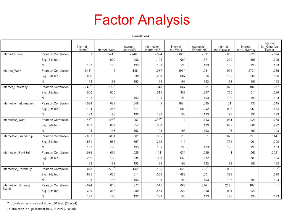
27 6. Interpretation: Component Matrix (factor loadings) –The most relevant output of a factorial analysis is the so called “component matrix”, which shows the correlations between the original input variables and the obtained components (factor loadings) –Each variable is associated specifically to the factors (components) with which there is the highest correlation –The interpretation of the each factor has to be guided considering the variables with the highest correlations related to single factor Factor Analysis

28 6. Interpretation: Correlation between Input Vars & Factors The new Factors must have a meaning based on the correlation structure

29 6. Interpretation: The correlation structure between Input Vars & Factors In this case the correlation structure is well defined and the interpretation phase is easier

30 Issues of the Factor Analysis are the following: a) How many Factors (or components) need to be considered 6. The degree of the interpretation of the components and how they affect the next analyses b) How to interpret 1.The correlation between the principal components and the original variables 2.The rotation of the principal components Factor Analysis

31 6. Interpretation: The rotation of factors –There are numerous outputs of factorial analysis which can be produced through the same input data –These numerous outputs don’t provide interpretation that are remarkably different from one another, as matter of fact they differ only slightly and there are areas of ambiguity Factor Analysis

32 x3x3 x4x4 CF i CF j x1x1 x2x2 The coordinates of the graph are the factor loadings Interpretation of the factors Interpretation of the factors CF* i CF* j Factor Analysis

33 6. Interpretation: The rotation of factors –The Varimax method of rotation, suggested by Kaiser, has the purpose of minimizing the number of variables with high saturations (correlations) for each factor –The Quartimax method attempts to minimize the number of factors tightly correlated to each variable –The Equimax method is a cross between the Varimax and the Quartimax –The percentage of the overall variance of the rotated factors doesn’t change, whereas the percentage of the variance explained by each factors shifts Factor Analysis

34 Analisi Fattoriale Before the rotation step

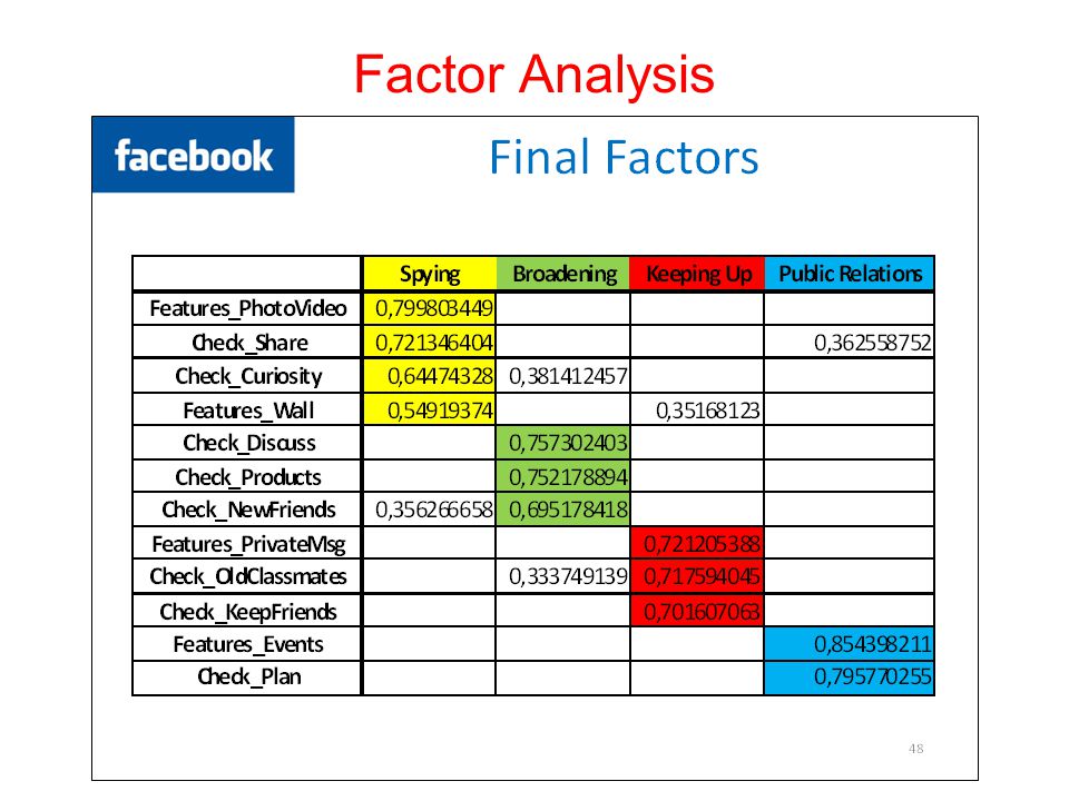
35 Analisi Fattoriale After the rotation step

36 5. Communalities: The communalities don’t change after the Rotation Step

37 6. Interpretation: The correlation structure between Input Vars & Factors improves after the rotation step

38 6. Interpretation: The correlation structure between Input Vars & Factors The variable with the lowest communality is not well explained by this solution

39 Once an adequate solution is found, it is possible to use the obtained factors as new macro variables to consider for further analyses on the phenomenon under investigation, thus replacing the original variables; Again taking into consideration the example, we may add six new variables into the data file, as follows: –Health, –Convenience & Practicality, –Image, –Handicraft, –Communication, –Taste. They are standardized variables: zero mean and variance equal to one. They will be the input for further analyses of Dependence or/and Interdependence. Factor Analysis

40 Indentification of the input variables Standardization P.C. methods first findings Number of factors Rotation Interpretation Factor Analysis