Lungo periodo e crescita

Presentazione sul tema: "Lungo periodo e crescita"— Transcript della presentazione:

1 Lungo periodo e crescita
Laboratorio di Macroeconomia lezione 2

2 Il lungo periodo Le fluttuazioni perdono rilevanza
Il PIL cresce (salvo shock come la crisi del o in caso di recessioni gravi) Per tutti?

3

4

5

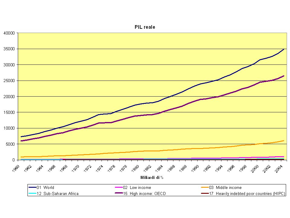
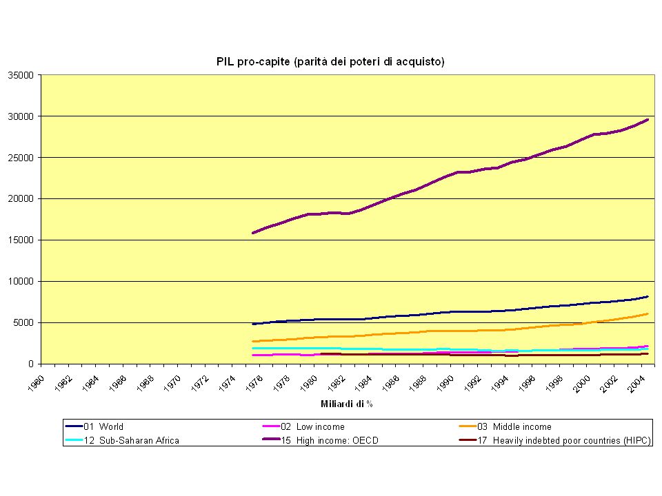
6 Crescita in diverse aree del mondo
Paesi OCSE – la crescita tende a convergere Asia – alcuni paesi (Singapore, Taiwan, Corea del Sud) sono cresciuti rapidamente, passando da circa il 16% del PIL USA nel 1960 al 65% di oggi. La Cina è al 50% Africa – per paesi molto poveri nel 1960 la situazione è addirittura peggiorata (Niger), oggi il PIL del Niger è la metà di quello del 1960. La crescita non è automatica: quali sono i fattori?

7 Funzione di produzione aggregata
Y=F(K,N) (in realtà capitale e lavoro non sono omogenei) F dipende dallo stato della tecnologia Rendimenti di scala Crescenti Costanti Decrescenti In generale, capitale e lavoro hanno rendimenti decrescenti

8 RENDIMENTI DECRESCENTI DEL CAPITALE
Prodotto e capitale per occupato (modello di crescita esogena di Solow) Y/N=F(K/N,N/N)=F(K/N,1) Y/N Miglioramento tecnologia RENDIMENTI DECRESCENTI DEL CAPITALE K/N

9 Fattori di crescita Aumento del capitale per occupato (risparmio)
Miglioramento della tecnologia Il solo aumento del capitale non permette di sostenere la crescita, serve progresso tecnologico

10 Crescita e benessere Non c’è un’equazione crescita=felicità
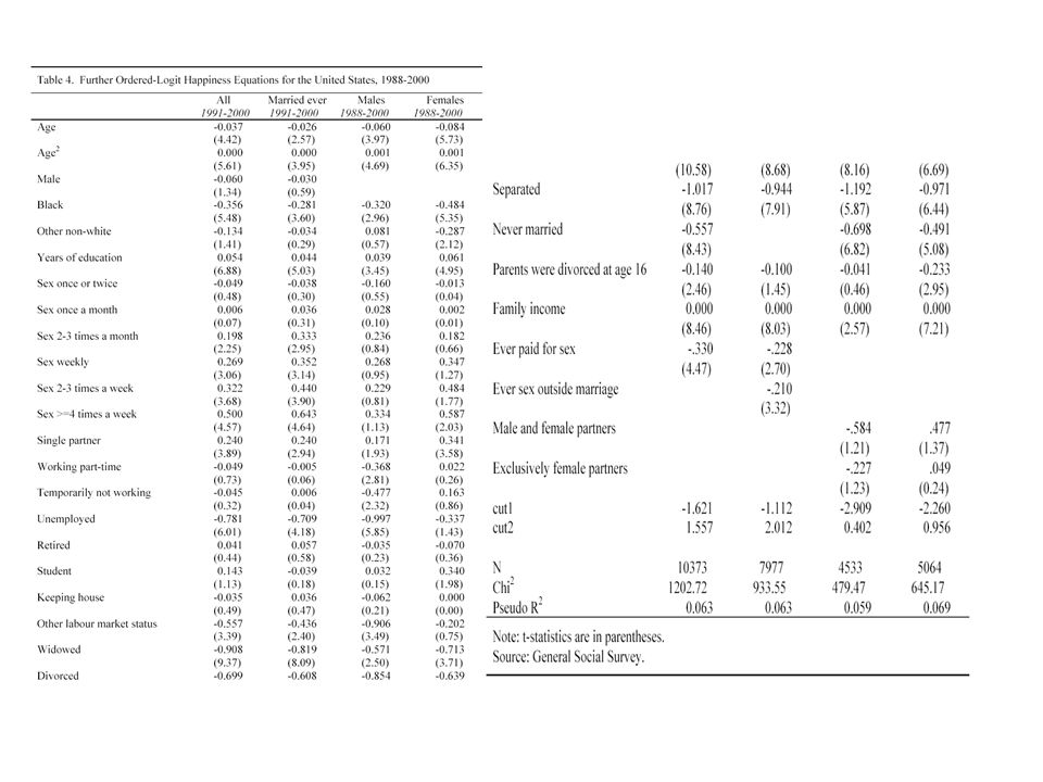
Recentemente, gli economisti hanno cercato di quantificare la felicità (o meglio il well-being) David G. Blanchflower, Andrew J. Oswald (2004). Well-being over time in Britain and the USA. Journal of Public Economics 88 (2004) 1359– 1386 Declino felicità in USA, stabilità in UK David G. Blanchflower, Andrew J. Oswald (2004). MONEY, SEX AND HAPPINESS: AN EMPIRICAL STUDY. NBER Working Paper 10499

11 Quantificazione del “well-being”

12

13 Il rapporto Stern www.hm-treasury.gov.uk
evidence gathered by the Review leads to a simple conclusion: the benefits of strong, early action considerably outweigh the costs. The evidence shows that ignoring climate change will eventually damage economic growth. Our actions over the coming few decades could create risks of major disruption to economic and social activity, later in this century and in the next, on a scale similar to those associated with the great wars and the economic depression of the first half of the 20th century. And it will be difficult or impossible to reverse these changes. Tackling climate change is the pro-growth strategy for the longer term, and it can be done in a way that does not cap the aspirations for growth of rich or poor countries. The earlier effective action is taken, the less costly it will be.

14

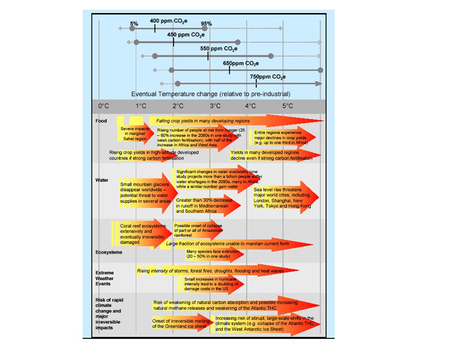
15 “Business as Usual”: Impatto sui costi

16 In sintesi Extreme weather could reduce global gross domestic product (GDP) by up to 1% A two to three degrees Celsius rise in temperatures could reduce global economic output by 3% If temperatures rise by five degrees Celsius, up to 10% of global output could be lost. The poorest countries would lose more than 10% of their output In the worst case scenario global consumption per head would fall 20% To stabilise at manageable levels, emissions would need to stabilise in the next 20 years and fall between 1% and 3% after that. This would cost 1% of GDP

17 Cambiamento climatico: i fatti
Metoffice.co.uk Fact 1: Climate change is happening and humans are contributing to it Fact 2: Temperatures are continuing to rise Fact 3: The current climate change is not just part of a natural cycle Fact 4: Recent warming cannot be explained by the Sun or natural factors alone Fact 5: If we continue emitting greenhouse gases this warming will continue and delaying action will make the problem more difficult to fix Fact 6: Climate models predict the main features of future climate

18 Peter A. Stott, F. B. Tett, G. S. Jones, M. R. Allen, J. F. B
Peter A. Stott, F. B. Tett, G. S. Jones, M. R. Allen, J. F. B. Mitchell, G. J. Jenkins (2000), External Control of 20th Century Temperature by Natural and Anthropogenic Forcings, Science, Vol no. 5499, pp

19 I dati (1994) The authors present global fields of decadal annual surface temperature anomalies, referred to the period , for each decade from to and for In addition, they show decadal calendar-seasonal anomaly fields for the warm decades and The fields are based on sea surface temperature (SST) and land surface air temperature data. The SSTs are corrected for the pre-World War II use of uninsulated sea temperature buckets and incorporate adjusted satellite-based SSTs from 1982 onward. These results extend those published in the 1990 Intergovernmental Panel on Climate Change Scientific Assessment. Despite poor data coverage initially and around the two World Wars the generally cold end of the nineteenth century and start to the twentieth century are confirmed, together with the substantial warming between about 1920 and Slight cooling of the northern hemisphere took place between the 1950s and the mid-1970s, although slight warming continued south of the equator. Recent warmth has been most marked over the northern continents in winter and spring, but the 1980s were warm almost everywhere apart from Greenland, the northwestern Atlantic and the midlatitude North Pacific. Parts of the middle- to high-latitude southern ocean may also have been cool in the 1980s, but in this area the climatology is unreliable. The impact of the satellite data is reduced because the record of blended satellite and in situ SST is still too short to yield a climatology from which to calculate representative anomalies reflecting climatic change in the southern ocean. However, the authors propose a method of using existing satellite data in a step toward this target. The maps are condensed into global and hemispheric decadal surface temperature anomalies. The authors show the sensitivity of these estimated anomalies to alternative methods of compositing the spatially incomplete fields.

20

21 I dati pubblicamente disponibili
Hadley Centre, temperatures in Central England on 20 May

22 Anomalie temperature negli ultimi 10 anni
Tra il 1997 and 2007, la temperatura del 20 maggio è stata sopra la media in 8 anni su 11 Statisticamente, la probabilità di 8 valori su 11 sopra la media è circa l’8% Statisticamente è difficile dire che siano dati anomali

23 Risparmio, capitale e crescita
Il tasso di risparmio influisce sulla crescita solo nel breve periodo S + T = I + G I = S + (T – G), dove (T – G) è il risparmio pubblico Se T – G = 0 e S=sY allora I=S=sY Gli investimenti dipendono dal tasso di risparmio

24 Investimento e capitale
L’investimento è un flusso (annuale) Il capitale è uno stock (accumulato) che si deprezza (ammortamenti) Kt = (1-d) Kt-1+It

25 La relazione tra accumulazione del capitale, risparmio e produzione
Kt = (1-d) Kt-1+It Kt / N = (1-d) Kt-1 / N + sYt / N Kt / N – Kt-1 / N = sYt / N - d Kt-1 / N La variazione di capitale per occupato dipende dal risparmio, dalla produzione e dagli ammortamenti

26 Lungo periodo e stato stazionario
Nel lungo periodo (lunghissimo), la produzione per addetto e il capitale per addetto convergono a valori costanti Nel cosidetto “stato stazionario”, il capitale non varia più e si stabilizza al valore K* K* / N – K* / N = sYt / N - d K* / N = 0 quindi sYt / N = d K* / N ovvero sF(K* / N) = K*/N inoltre Y* / N = F(K* / N,s)

27 In sintesi, nel modello di crescita “esogena”
Nel lungo periodo: Il livello di produzione dipende dalla quantità di capitale Il tasso di crescita del prodotto per addetto è nullo Il tasso di risparmio non ha effetti sulla crescita Il tasso di risparmio influenza il livello di produzione per addetto nel lungo periodo, ma non la crescita

28 Politiche sul tasso di risparmio
Creare un avanzo di bilancio Sgravi fiscali per i risparmiatori Nel breve periodo l’aumento del risparmio è legato ad una riduzione dei consumi Nel lungo periodo, i consumi aumentano (e raggiungono il loro livello massimo) solo se il risparmio è pari al valore definito “livello di capitale di regola aurea” (golden rule)

29 Capitale fisico e capitale umano
Y/N = f(K/N, H/N) H: livello di capitale umano per addetto L’aumento del capitale umano aumenta la produttività Il “capitale umano” si misura generamente attraverso i salari Le ipotesi sono uguali a quelle sul capitale fisico Il flusso è l’educazione, il capitale umano è lo stock

30 RENDIMENTI DECRESCENTI DEL CAPITALE UMANO?
Y/N Educazione (= investimenti) RENDIMENTI DECRESCENTI DEL CAPITALE UMANO? H/N

31 Y/N e crescita Un paese che :
Risparmia Investe in ricerca tecnologica Investe in educazione giungerà ad un prodotto pro capite più elevato (ma la crescita maggiore non verrà sostenuta nel lungo periodo e si stabilizzerà) La crescita è “finita”? Teoria della crescita endogena Aumentando capitale umano e fisico simultaneamente, la crescita potrebbe non essere “limitata”, ma infinita

32 Il progresso tecnologico
Y = F (K, N, A) A = stato della tecnologia Ad esempio: Y = F(AK, AN) in cui la “tecnologia” aumenta il peso del fattore lavoro e di quello capitale… Servono meno lavoratori\capitale per produrre la stessa quantità Gli stessi lavoratori\capitale producono di più Dividendo per AN si procede come in precedenza

33 Determinanti del progresso tecnologico
Attività di ricerca e sviluppo Fertilità di R&S Appropriabilità di R&S (brevetti)

34 Sito interessante… Grafici principali variabili macro per paesi sviluppati: Simulazione modelli macroeconomici

35 Il processo di Lisbona Risposta alla bassa produttività e alla stagnazione della crescita Obiettivi fissati nel 2000, realizzati nel 2010 (lungo periodo?) Innovazione come motore della crescita “Economia che impara” (educazione, lauree tecnologiche) Rinnovamento sociale ed ambientale

36 Obiettivi generali

37 Esempio di obiettivi specifici

38 Il “rilancio” (2005)

39 Possibili tesi… Costi della crescita e distribuzione internazionale
Processo di Lisbona e… Crescita, efficienza e progresso tecnologico in un determinato paese Crescita e sostenibilità Spillover Il ruolo dell’ingegneria genetica nella crescita dei paesi in via di sviluppo Corruzione, burocrazia e sviluppo

40 Crescita, progresso ed efficienza
This paper analyzes productivity growth in 17 OECD countries over the period A nonparametric programming method (activity analysis) is used to compute Malmquist productivity indexes. These are decomposed into two component measures, namely, technical change and efficiency change. We find that U.S. productivity growth is slightly higher than average, all of which is due to technical change. Japan's productivity growth is the highest in the sample, with almost half due to efficiency change.

41 Crescita sostenibile The Scandinavian Journal of Economics
Volume 99 Page 1 - March 1997 doi: / Volume 99 Issue 1 Sustainability and Technical Progress Martin L. Weitzman A rigorous model connects together the following three basic concepts: (1) "sustainability" — meaning the generalized future power of an economy to consume over time; (2) "Green NNP" — meaning a current measure of national income that subtracts off from GNP not just depreciation of capital but also, more generally, depletion of environmental assets evaluated at current efficiency prices; (3) "technological progress" — meaning a projection onto the future of the so-called "Solow residual". A simple general formula is derived. Some crude calculations suggest a possibly strong effect of the residual, which hints that our best present estimates of long-term sustainability may be largely driven by predictions of future technological progress.

42 Spillover

43 OGM, ricerca e paesi in via di sviluppo
Poorer nations turn to publicly developed GM crops JI Cohen - Nature Biotechnology, 2005

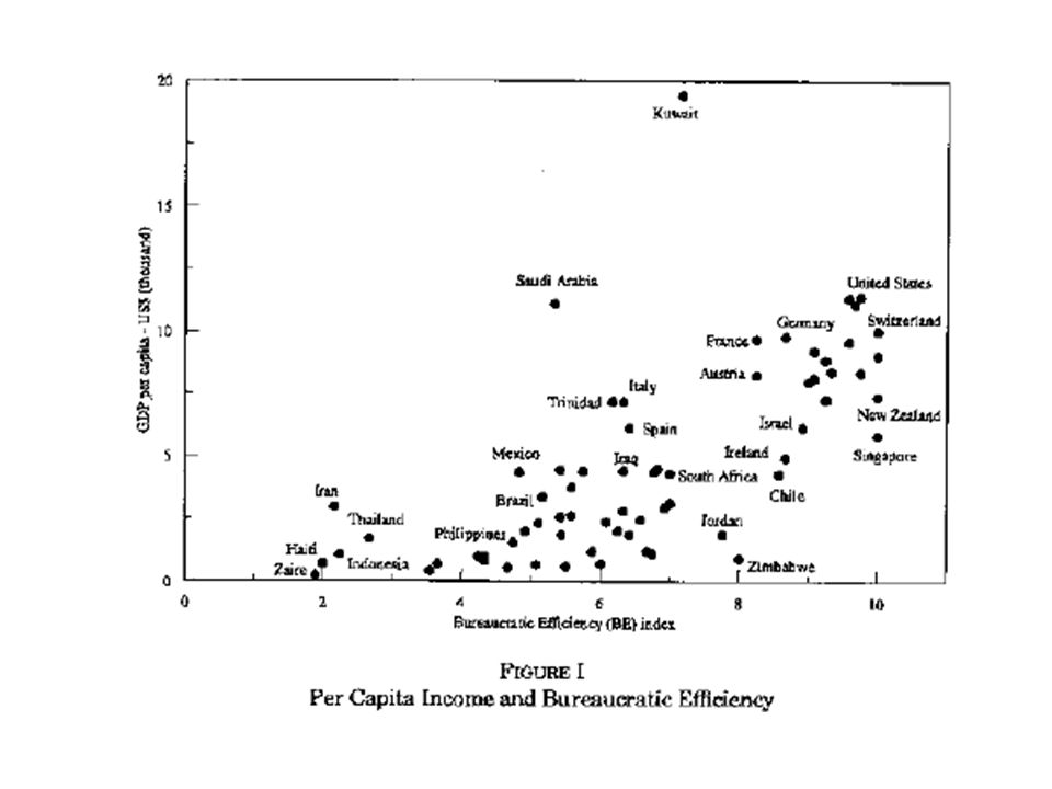
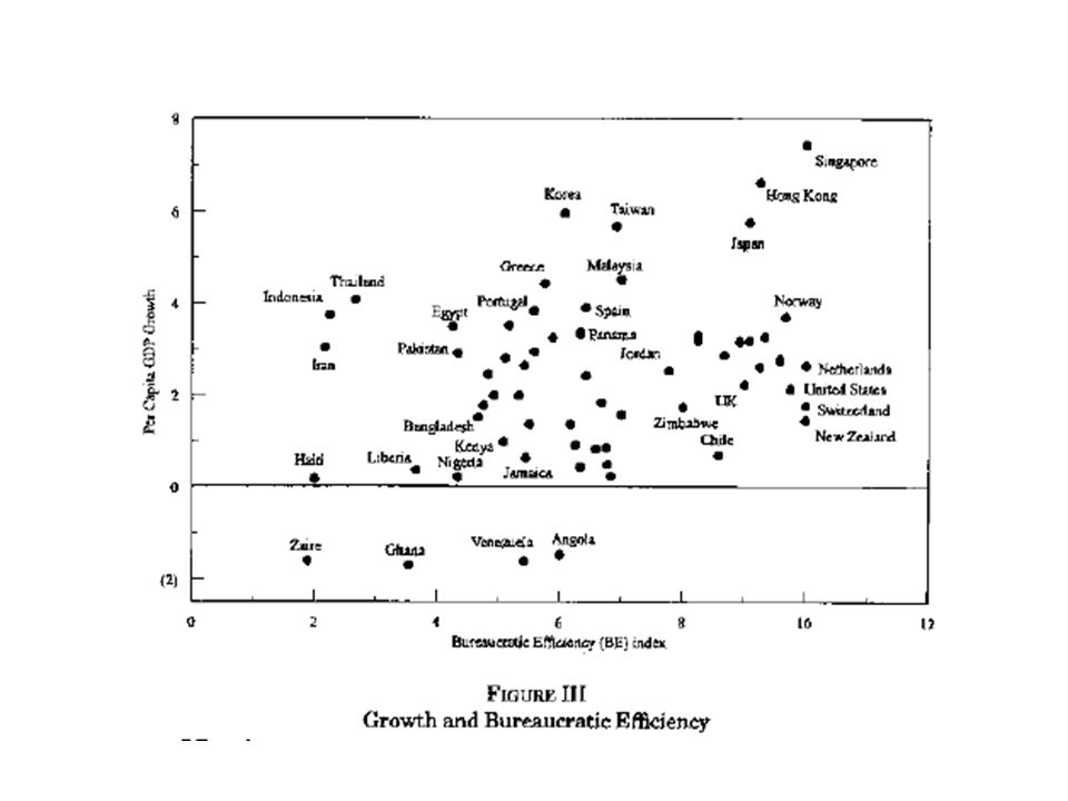
44 Corruption and Growth Paolo Mauro
The Quarterly Journal of Economics, Vol. 110, No. 3. (Aug., 1995), pp This paper analyzes a newly assembled data set consisting of subjective indices of corruption, the amount of red tape, the efficiency of the judicial system, and various categories of political stability for a cross section of countries. Corruption is found to lower investment, thereby lowering economic growth. The results are robust to controlling for endogeneity by using an index of ethnolinguistic fractionalization as an instrument.

45

46 Efficienza burocratica

47

48

49 Progresso tecnico, bioenergie e prezzi del pane
L’innovazione tecnologica che ha portato ai biocombustibili che effetti avrà? Becker: se l’aumento dei prezzi è dovuto alla pressione della domanda, allora l’offerta si adeguerà attraverso un aumento della produttività e al progresso tecnologico… biotecnologie?