La validità di un test diagnostico

Presentazione sul tema: "La validità di un test diagnostico"— Transcript della presentazione:

1 La validità di un test diagnostico
Prof. Roberto de Marco Sensibilità e specificità Confronto tra differenti test diagnostici Determinazione della soglia ottimale del test

2 Latency period Induction period

3 Prevenzione primaria, secondaria e terziaria
Prima che si instauri la malattia: Prevenzione primaria = Rimozione dei fattori di rischio (ad esempio, campagne contro il fumo o contro l’alcoolismo) o riduzione degli effetti dell’esposizione (vaccinazioni). La malattia si è instaurata, ma non è ancora evidente dal punto di vista clinico: Prevenzione secondaria = Individuazione precoce dei casi tramite uno screening (ad esempio, Pap test per il tumore dell’utero, mammografia per il tumore del seno, sangue occulto nelle feci per il tumore del colon). La malattia si è manifestata clinicamente: Prevenzione terziaria = Terapia appropriata e riabilitazione per prevenire o ridurre le conseguenze negative della malattia stessa (ad esempio, assistenza agli infartuati e riabilitazione).

4 Screening 1) Somministrazione di un test diagnostico poco costoso e poco invasivo a larghi settori della popolazione a rischio per una determinata patologia per identificare gli individui ammalati prima che la malattia si riveli dal punto di vista clinico. Lo scopo dello screening è diagnosticare precocemente la malattia, quando è ancora curabile, per ridurne la mortalità e morbilità

5 Survival time after diagnosis – lead time
Pre-detectable Detectable, preclinical Clinical Disability or death Age: Lead time A successful screening program will advance the time of detection from the point at which symptoms appear (when the disease is likely to be detected clinically) to some earlier point in the natural history of the condition. The time by which detection is advanced is sometimes called the lead time. The lead time provides the opportunity for treatment to gain the upper hand over the disease. The lead time also provides the opportunity for screening to appear to be effective when in fact it produces no benefit. This possibility, called “lead time bias”, is illustrated on the following slide. Possible detection via screening Clinical detection 9/10/2002 Natural history; population screening

6 Classificazione dei soggetti in
Obiettivo del test: Classificazione dei soggetti in POSITIVI (alta probabilità di essere malati) NEGATIVI (alta probabilità di essere sani) Screening utili agli individui: Screening per il tumore al collo dell’utero (PAP test) via esame citologico Screening per il tumore della mammella via mammografia in donne di età >50 Screening utili alla collettività: Test cutaneo con tubercolina Screening per l’infezione streptococcica per prevenire la febbre reumatica

7 SCREENING

8 EX: Mammography Pt.s in early stages respond well to treatment
Patients with advanced disease do poorly Earlier diagnosis, better chance of survival Mammography is tool for early detection

9 Mammography: Risk v. Benefit
Breast cancer in United States in 2009 (estimated): New cases: 192,370 (female); 1,910 (male) Deaths: 40,170 (female); 440 (male) Us population 306 million in deaths /million Mortality risk from mammography induced radiation is 5 deaths/ million pts. using screen film mammography More risky to refuse mammography!

10 Based on review of RCTs SCREENING BENEFITS
Screening mammography mortality reductions were 15% for women in their 40s 14% for women in their 50s 32% for women in their 60s US Preventive Service Task Force (USPSTF)

11 Harms of Screening: Additional Intervention
For every 1000 mammograms women (8-10%) asked to return for addition evaluation 45-65 told that there is nothing of concern 20 are asked to return in 6 months Probably benign (<2% prob of malignancy) 15 (1-2%) recommended to have a biopsy 2 to 5 will have cancer 10-13 have benign biopsy Davey MS about…/breastscreening.ppt

12 popolazione malati test + falsi positivi negativi veri

13 Validità di un test di screening
Falsi positivi GOLD STANDARD malati sani a b Test + c d Test - a+c b+d Falsi negativi

14 malati a c sani d a+c b+d malati a c sani d a+c b+d
Sensibilità: probabilità che un test sia positivo nei malati malati a c sani b d Test + Test - a+c b+d Sen=pr(T+|M+) Sen=a/(a+c) Specificità: probabilità che un test sia negativo nei sani malati a c sani b d Test + Test - a+c b+d Spe=pr(T-|M-) Spe=d/(b+d)

15 Scelta del livello ottimale di sensibilità e specificità:
Dipende da: Considerazioni cliniche sulla malattia in studio Obiettivo dell’intervento Malattie molto rare Alta sensibilità (per non rischiare di perdere i pochi casi) Malattie molto letali e l’intervento nelle fase precoci può permettere un aumento della sopravvivenza o una miglior prognosi Alta sensibilità Se l’intervento successivo alla diagnosi non modifica di molto la storia naturale della malattia Bassa percentuale di falsi positivi Studi epidemiologici Bassa percentuale di falsi positivi

16 malati a c sani d a+c b+d malati a c sani d a+c b+d
Valore predittivo nei positivi (V+): probabilità che chi ha il test positivo sia malato malati a c sani b d Test + Test - a+c b+d V(+)=pr(M+|T+) V(+)=a/(a+b)* Valore predittivo nei negativi (V-): probabilità che chi ha il test negativo sia sano malati a c sani b d Test + Test - a+c b+d V(-)=pr(M-|T-) V(-)=d/(c+d)* * Formule valide solo nel caso di un campione random classificato contemporaneamente rispetto al test e al gold standard

17 Esercizio: si considerino:
individui asintomatici di cui affetti da M+ Sensibilità=90% Specificità=90% Calcolare il numero di veri positivi e di falsi positivi e il valore predittivo che ci si aspetta in questa popolazione di individui Qual è la prevalenza della malattia? Qual è la prevalenza della malattia misurata da questo test di screening? M+ M- T+ T- VP=Sen*10000=0.90*10000=9000 VN=Spe*90000=0.90*90000=81000 9000 9000 18000 FP= =9000 1000 81000 82000 V(+)=90000/18000=50% 10000 90000 100000 PREV=10000/100000=0.1=10% PREV(test)=18000/100000=18%

18 Esercizio: cont Si calcolino il numero di falsi positivi, di falsi negativi e il valore predittivo positivo nel caso in cui lo stesso test venga sottoposto a un gruppo di popolazione che ha una prevalenza del 30%- Confrontate i risultati e commentate

19 Example: Mammography screening of unselected women
Disease status Cancer No cancer Total Positive ,117 Negative , ,342 Total , ,459 Prevalence = 0.3% (179 / 63,459) Se = 73.7% Sp = 98.4% PV+ = 11.8% PV– = 99.9% Source: Shapiro S et al., Periodic Screening for Breast Cancer The above table shows data from the classic randomized trial of breast cancer screening conducted by Shapiro and colleagues in New York City’s Health Insurance Plan (HIP). The table is taken from Leon Gordis’ textbook. The prevalence of breast cancer is less than 1%, and even with specificity of greater than 98% only 11.8% of the women with a positive mammogram actually had breast cancer (PPV=11.8%). Note that in a actual screening program, only people with a positive test undergo a diagnostic work-up. From the results we can learn the numbers of true positives and false positives, which permit us to calculate positive predictive value. Estimating sensitivity and specificity is more problematic, since we do not know how many cases were missed, i.e., the number of false negatives. We can estimate that number based on the number of people who develop the disease soon after being screened, but you can see why that method leaves something to be desired. Without knowing the number of false negatives we cannot determine the exact number of true negatives. For this reason, Gordis’ textbook says that sensitivity and specificity cannot be estimated from the results of a screening program. However, if we have a good estimate of the prevalence of the disease or at least know that it is very low, then we can often make a good estimate of the specificity based on the number of false positives and the estimated number of cases (and therefore of non-cases) based on disease prevalence. Note that a small inaccuracy in the denominator of the specificity will not alter the numerical result nearly as much as will a small inaccuracy in the denominator of the sensitivity estimate.

20 Sensitivity = 93%, Specificity = 92%
Effect of Prevalence on Positive Predictive Value Sensitivity = 93%, Specificity = 92% Surgical biopsy (“gold standard”) Cancer No cancer Prev. Without palpable mass in breast Fine needle Positive % aspiration Negative With palpable mass in breast Fine needle Positive % aspiration Negative PV+ = 64% To provide a taste of clinical epidemiology, for those who would like it, here are possible results from the use of final needle aspiration to evaluate a suspected breast cancer. The table compares the results from fine needle aspiration with the determination of cancer based on a surgical biopsy, whose results are regarded as definitive. The upper portion of the table shows the data for women with a positive mammogram but no palpable breast mass. 13% of these women actually have breast cancer. The PV+ is 64%. The lower portion of the table shows women with a palpable breast mass. Here, 38% of the women have breast cancer, and the PV+ is considerably greater, at 88%. The prevalence is referred to as the “prior probability” or “pretest probability”, since it represents the probability that a randomly selected women has cancer. The PV+ is referred to as the “posttest probability” or “posterior probability”, since it represents the probability that a woman with a positive test has cancer. The higher the ratio of the posterior to the prior probability, the more informative the test. In clinical medicine, the informativeness of a diagnostic test is quantified by its likelihood ratio. The likelihood ratio of a positive test is the ratio of the sensitivity of the test to its false positive rate (1 – specificity). It turns out that this ratio equals the ratio of the posterior odds to the prior odds (recall that the odds are simply the ratio of the probability to its inverse). The greater the likelihood ratio of a positive test, the more likely it is that a positive test indicates the presence of the condition. (More: or a clinical epidemiology textbook such as the ones by David Sackett et al., Robert Fletcher et al., or Raymond Greenberg et al.) PV+ = 88% See

21 La maggior parte dei test dignostici produce un risultato quantitativo
Per discriminare tra sani e malati è necessario disporre di un valore soglia o cut off Situazione ideale: sani e malati restituiscono valori del test differenti Cut off immediatamente determinato Situazione reale: sovrapposizione nella distribuzione di sani e malati

22 Esempio:

23 Sensibilità e specificità sono antagoniste
Sensibilità e specificità sono antagoniste. A parità di strumento diagnostico, ogni aumento nella sensibilità comporta una diminuzione nella specificità. Quando il costo dei falsi positivi uguaglia quello dei falsi negativi, la scelta del cut-off ottimale può essere ottenuta da criteri statistici.

24 GRAFICO DEL LIVELLO DECISIONALE
Indice di Youden: Sen+Spe-1 Indice di Youden

25

26 Utilizzati per rappresentare
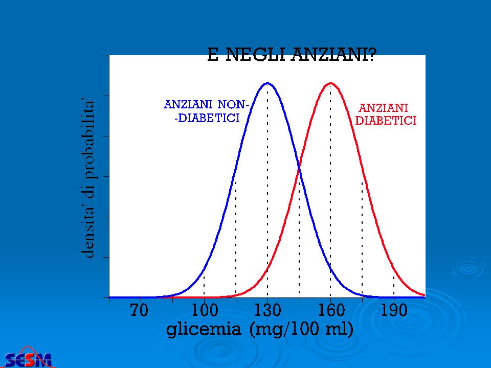
Come variano sensibilità e specificità al variare del cut off? I ESEMPIO (PAZIENTI DIABETICI) II ESEMPIO (PAZIENTI DIABETICI ANZIANI) specificità 1 - sensibilità Cut-off 50.0 % % 100 mg/dl 2.3 % 97.7 % 84.1 % 15.9 % 99.9 % 115 mg/d l 130 mg/dl 0.1 % 145 mg/dl 0.003 % 160 mg/dl --- 175 mg/dl Utilizzati per rappresentare le CURVE ROC

27 (Receiver operating characteristic)
Le curve ROC (Receiver operating characteristic) diabetici giovani diabetici anziani 130 mg 145 mg 160 mg 175 mg

28 Esercizio: la tabella riporta i risultati del test ELISA per HTLV-III tra pazienti con AIDS e donatori di sangue sani (Weiss et al., 1985): per ogni valore del cut off sono specificati i pazienti che risultano negativi al test. Calcolare per ognuno dei valori del test i livelli di specificità e sensibilità Valutare, in base al valore dell’indice di Youden, qual è il valore soglia ottimale. .

29 L’indice di Youden permette di ottenere quel valore soglia che minimizza la probabilità trovare falsi positivi e falsi negativi: Nel nostro caso, tale valore è pari a 3

30 La signora è figlia di una portatrice nota
La signora R.P ha 24 anni. Uno dei suoi fratelli e uno zio materno sono affetti da emofilia; suo padre e un altro fratello ne sono immuni. La signora non presenta emofilia manifesta. Sottoposta al test di Riza essa risulta positiva. Qual è la probabilità che essa sia una portatrice? probabilità a priori: P(H1:)=0.5= p La signora è figlia di una portatrice nota probabilità a priori: P(H0:)=1-0.5=1- p Sen=0.94 Spe=0.82 Prob. che il test sia positivo se la signora è portatrice prob. che chi ha il test positivo sia portatore

31 Talvolta la validità di uno strumento di misura non può essere stabilita (assenza di un gold standard). In tal caso è necessario che almeno la sua affidabilità (riproducibilità) sia buona!

32 MISURA DELLA RIPRODUCIBILITA’ TRA DUE OPERATORI
osservatore 1 + - a b c d R1 + oservatore 2 - R2 C1 C2 N a+d Po = = observed proportion of agreement N R1C1 R2C2 expected proportion of agreement by chance Pe = = + 2 N 2 N Po - Pe K = 1 - Pe Se(K) = 2

33 RETINOPATIA MODERATA / SEVERA
CONCORDANZA TRA 2 CLINICI NELL’ESAMINARE LO STESSO GRUPPO DI 100 FOTO DEL fondo oculare SECONDO CLINICO RETINOPATIA ASSENTE MODERATA / SEVERA PRIMO CLINICO RETINOPATIA ASSENTE 46 10 56 RETINOPATIA MODERATA / SEVERA 12 32 44 58 42 100  CONCORDANZA OSSERVATA = = 78% 100  CONCORDANZA ATTESA in base al caso 56 x 58 attesi per la cella a = = 32,5 100 44 x42 attesi per la cella d = = 18,5 100 Exp(a) + Exp(d) 32,5 + 18,5 = = 51%  CONCORDANZA dovuta al caso = totale 100

34 0% 100% ASSENZA DI CONCORDANZA COMPLETA CONCORDANZA CONCORDANZA OSSERVATA = 78% 100 CONCORDANZA ATTESA in base al caso CONCORDANZA non dovuta al caso 32,5 + 18,5 78% - 51% = 27% = 51% 100 Cohen’s kappa is thus the agreement adjusted for that expected by chance. It is the amount by which the observed agreement exceeds that expected by chance alone, divided by the maximum which this difference could be POTENZIALE CONCORDANZA non dovuta al caso 100% - 51% = 49% CONCORDANZA OSSERVATA non dovuta al caso 27% KAPPA = = = 55% CONCORDANZA POTENZIALE non dovuta al caso 49%

35 Concordanza osservata (P0) e K di Cohen (
Concordanza osservata (P0) e K di Cohen (*) nella risposta alle stesse domande di un questionario di screening in due occasioni temporalmente vicine sintomi P0 K+ K- K C.I. (90%) 1) sibili .90 .61 .94 .56 1.1) Con mancanza di respiro .96 .34 .95 .22 1.2) senza raffreddore .93 .58 .54 2) Costrizione .30 17-.43 3) Mancanza di respiro .92 .51 .47 4) Attacco di tosse .74 .81 .38 5) Asma .98 .75 .99 .76 6) Farmaci per asma .50 .49 7) Raffreddore allergico .91 .77 .72 Valori di riferimento (Londis J.R. Koch G.G., Biometrics 1977; 33: ) Valori di K concordanza K<.40 scarsa .40 < K < .60 moderata .60 < K < .80 notevole K > .80 quasi perfetta